
In Solid Angle and the Rendering Equation, the analysis centered on the integration measure: while path tracers sample directions over solid angle , surface irradiance and the projected rendering equation integrate against projected solid angle . For planar polygonal sources such as a rectangle, practical Monte Carlo sampling routines draw points uniformly across surface area. Transforming this area density into a directional density requires the differential solid angle conversion:
Omitting the squared distance or the emitter normal foreshortening term yields an estimator that is strictly biased and non-convergent with increasing sample count .
As detailed in Importance Sampling: Phong Lobe vs Cosine, evaluating competing directional sampling distributions operates in . For a finite disk subtending an angular radius of , the corresponding subtended solid angle evaluates analytically to
To evaluate the area Jacobian empirically, we deploy a physical test configuration: the night inspection bench. The scene consists of a vertical rectangular softbox with an in-frame diffuser, a matte inspection bench, a diffuse white Lambert calibration card, and a matte reference vise inside an unlit enclosure.
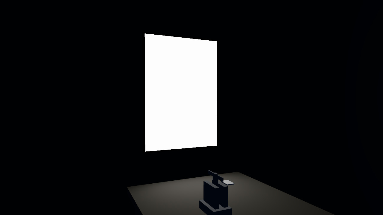
The diffuse card acts as the planar measurement receiver. Drawing uniform samples across the emitter parameterization yields an area probability density in ; mapping this quantity into incoming radiance integration requires scaling by the geometric Jacobian above.
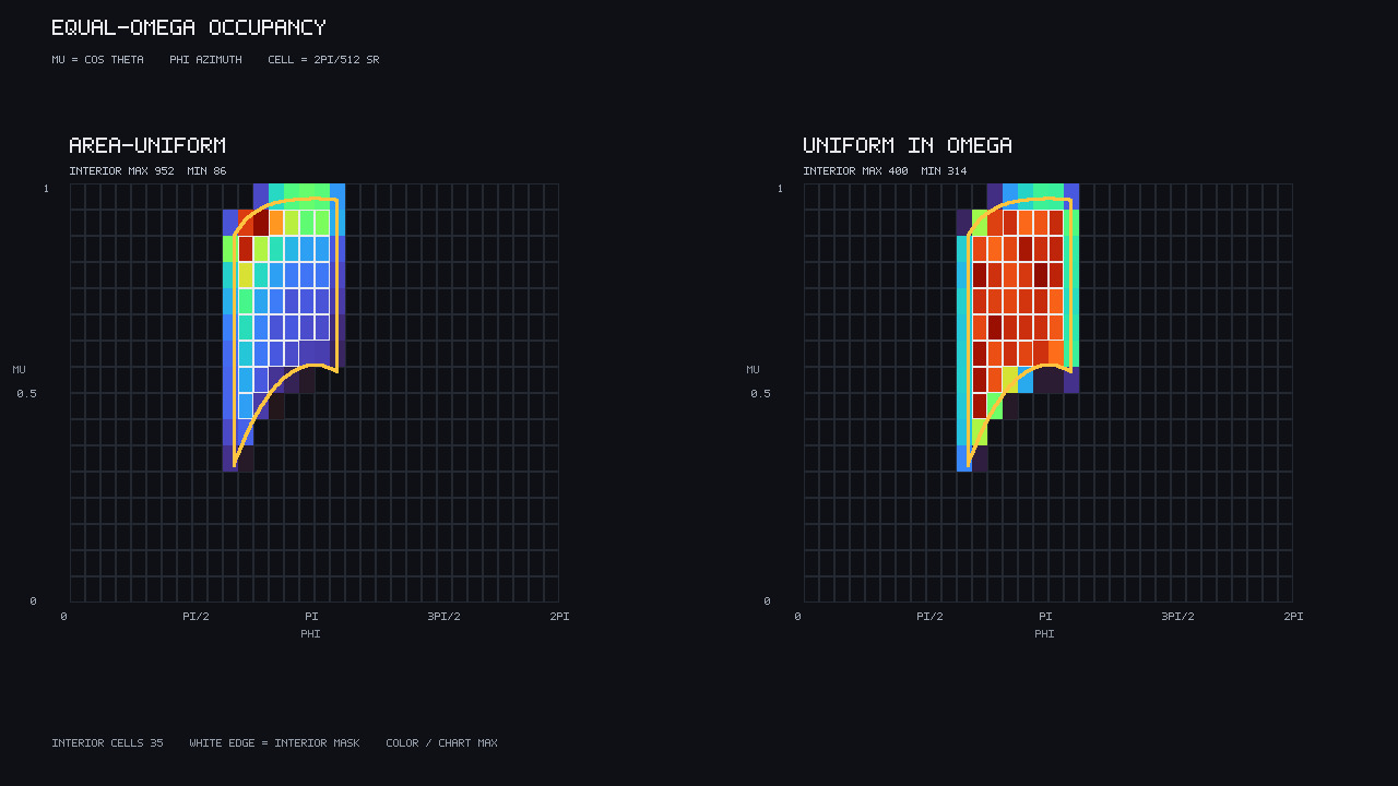
The directional distortion induced by area-uniform sampling is verified by measuring cell occupancy across the projected hemisphere. Using a discretized versus azimuth spherical grid with bin solid angles of , the rectangular panel projects across an interior mask of 35 cells. For an identical total sample count, an area-uniform generator produces an occupancy ranging from 86 to 952 samples per bin. Conversely, drawing uniformly within the subtended solid angle bounded by the source boundary constrains the distribution to 314..400 samples per bin.
Benchmark statistics were collected under Mesa 25.0.7 llvmpipe in linear Rec.709 using Khronos PBR Neutral () and pseudorandom seed 20260924:
| Parameter / Metric | Symbol / Field | Value |
|---|---|---|
| Projected solid angle | 0.419598441342 | |
| Surface irradiance | 1.67839376537 | |
| Centroid relative error | -0.194936551657 (rounded: -0.195) | |
| Panel-to-fill ratio | panel_over_fill |
22.0690362063 (or 22.069) |
| Distance ratio | (r_ratio) |
3.3491112796 (or 3.349) |
| Emitter Jacobian ratio | 37.5654619429 | |
| Source parameters | , , | , 0.80, 0.448 |
| Test suite status | assert |
72 pass / 0 fail |
Convergence of the unbiased legal estimator was tracked across shared prefixes: root-mean-square error decreased from 0.1644 to 0.1089, 0.06826, and 0.02638 at sample allocations . The precise values are:
rmse_legal_N16: 0.164412278931rmse_legal_N64: 0.108928582911rmse_legal_N256: 0.0682573241753rmse_legal_N1024: 0.0263804488107
Conversely, biased estimators converge to non-zero asymptotic floors at :
- Failure A (omitting ):
mean_rel_drop_r2_N1024 - Failure B (omitting ):
mean_rel_drop_cos_N1024
Photographic references and shop crops on the centroid evaluation plate are rendered with 8× supersampling box-filtered to 1280720 before tonemapping. Diagnostic occupancy distributions, bias plots, and the metrics readouts are rendered directly into native sRGB without supersampling.
Scene
The radiometric computations operate strictly in scene-referred linear Rec.709 with 1 shop, 1 rectangular source, and 1 Lambert receiver. Display mapping follows the configuration documented in Tone Mapping: Scene-Referred to Display-Referred: the Khronos PBR Neutral curve evaluated with parameters , , , and , followed by the IEC 61966-2-1 sRGB transfer function implemented on the CPU. Neutral determines output display code values but does not alter the underlying computed irradiance .
- Cover Presentation: The complete inspection bench environment showing the softbox, calibration card, and reference vise illuminated under verified area lighting and ambient shop fill. The image represents an un-annotated render without radiometric readouts.
- Occupancy Bins: The equal-solid-angle spherical discretization contrasting the area-uniform distribution against uniform solid angle generation across the 35 interior cells.
- Bias Characteristics: Relative RMSE computed across prefixes plotted against sample count . The legal sampling routine converges linearly on logarithmic axes, whereas estimators omitting geometric factors plateau at fixed asymptotic biases, with signed means tabulated at .
- Centroid Evaluation Plate: Side-by-side comparison of the full scene rendered via legal integration versus single-point centroid evaluation, marked with
CENTROID_SIGNED_REL-0.195,(EC-E)/E = -0.194937, andFROM THIS RUN. Regional crops of the card and bench show linear Rec.709 luminance values ofY 0.446(legal) andY 0.362(centroid) alongside an absolute error heat map derived directly from floating-point buffers prior to tonemapping. - Metrics Readout: A two-column visual log capture of runtime metrics; numerical values correspond verbatim to the accompanying analytical data.
Analytical evaluations should distinguish between tonemapped GLSL photographic renderings (subject to display transforms) and raw floating-point instrument measurements (occupancy bins, bias sweeps, and tabulated integral values).
Method
Equal- histogram
The spherical occupancy distribution empirically demonstrates the directional mapping distortion. The receiver hemisphere, centered on the surface normal , is parameterized using against a wrapped azimuthal angle . The parameterization domain is uniformly discretized into 16 steps in and 32 steps in :
This uniform grid—enforcing equal and equal —ensures identical solid angle subtension across all discrete cells, consistent with established derivations for spherical caps.
The evaluation contrasts two distinct spatial sampling populations, each utilizing draws evaluated independently from the irradiance estimator prefixes. The first configuration generates 16384 area-uniform samples directly on the diffuser surface, binning their resulting incident vectors . The second configuration generates directions uniformly via and , utilizing ray rejection against the spatial footprint until exactly 16384 valid diffuser intersections are accumulated. A discrete spherical cell is classified strictly as an "interior" cell if all 4 bounding corners maintain geometric intersection with the diffuser. While boundary bins containing partial intersections are rendered, quoted population extrema are rigorously constrained to the interior subset. This verified internal mask encompasses exactly 35 cells. Under the area-uniform generation strategy, the directional occupancy distribution exhibits high density variance spanning 86 to 952 samples. Conversely, the uniform-in- strategy maintains a tightly bounded interior occupancy of 314 to 400 samples.
The lower near edge of the physical emitter aligns with the global maximum of the area-to-directional Jacobian . Consequently, an equal- discrete cell mapping to this region corresponds to an extremely small differential surface area, resulting in severe under-sampling by the area-uniform generator. To maintain energy conservation, any stochastic intersection occurring within this domain requires an inversely proportional compensatory weight:
By contrast, the far spatial corner correlates with the global minimum of the Jacobian. Here, an equivalent equal- discrete cell subtends a dramatically larger differential surface area, thereby over-accumulating area-uniform ray hits that subsequently receive heavily diminished individual scalar weights. This mapping discrepancy mathematically dictates the 86-to-952 density disparity across the interior region. The uniformly drawn angular distribution appropriately stabilizes between 314 and 400. Local maximum normalization separates spatial density gradients from discrete boundary rasterization errors.
The drastic modulation of the compensatory weight is fundamentally dictated by radial distance . Across this specific spatial footprint, the geometric transfer kernel diverges by an absolute factor of 37.5654619429. Estimator formulations that omit this necessary scaling term reliably converge to an invalid radiometric integration target.
Discussion
Three failures
For a planar emitter with uniform exitant radiance and zero emission from the rear hemisphere, receiver irradiance is defined by integrating incoming radiance weighted by the geometric transfer kernel. The unbiased formulation accounts for both geometric foreshortening and inverse-square falloff. Systemic bias typically arises from three deviations:
- Failure A — Omission of the inverse-square law (): Preserving surface cosines and while omitting shifts the Monte Carlo expectation toward , altering the physical dimension of the estimator by . Because contributes maximal weight along the near boundary of the panel, omitting it severely underestimates total flux, yielding a relative mean error of -0.645746690189 at .
- Failure B — Omission of the emitter foreshortening term (): Omitting while retaining , the receiver cosine , and converges to . Because is already defined per unit projected area at the source, originates strictly from the differential area-to-solid-angle transformation rather than an emitter scattering lobe. While dimensionally consistent with irradiance, the integral evaluates the incorrect measure, converging to a relative error floor of +1.04013072615 at .
- Failure C — Single-point centroid approximation: Approximating the surface integral by evaluating the transfer kernel exclusively at the geometric centroid replaces numerical quadrature with a single distance and cosine pair scaled by total area . Because the measurement card is positioned near the panel's lower boundary and displaced from the center axis, this point-source approximation produces a large discrepancy relative to the true boundary integral, yielding (displayed as -0.195).
The receiver foreshortening term remains active across all test cases. An additional evaluation arm testing redundant weighting of introduced a dimensionless attenuation bias, converging to mean_rel_double_N1024 at .
Because tonemapping non-linearities and display transforms compress dimensional discrepancies, biased Monte Carlo estimators cannot be reliably evaluated from tonemapped photographic images alone. Numerical error floors are properly verified through raw floating-point error metrics on the bias plate, whereas the dimensionally consistent centroid approximation is analyzed on the centroid plate.
Change of measure
We first formalize the notation and physical quantities utilized in the subsequent evaluations.
| symbol | meaning | unit |
|---|---|---|
| instrument point on the card, | ||
| sample point on the diffuser | ||
| diffuser centroid, | ||
| , from the card toward the panel | unitless | |
| card normal, | unitless | |
| diffuser outward normal, | unitless | |
| unitless | ||
| unitless | ||
| means in the opening formula | ||
| means in the opening formula | ||
| diffuser area, | ||
| on the diffuser, else | ||
| constant one-sided radiance, | linear Rec.709 | |
| shop fill on the rest of the hemisphere, | linear Rec.709 | |
| card albedo, | unitless | |
| irradiance at from the diffuser alone | ||
| outgoing radiance of the Lambert card, | linear Rec.709 |
The two cosine terms parameterize distinct foreshortening effects. The receiver cosine is evaluated with respect to the direction from the measurement card toward the emitter, whereas the emitter cosine evaluates the direction from the emitter toward the card. Evaluating the dot product with respect to a shared direction vector naturally necessitates a sign inversion. Given the geometric configuration of the panel and card, both cosines remain positive for all valid surface samples. The computed numerical minima are and .
The one-sided diffuser occupies the plane , bounded by and . The domain spans a width of and a height of , yielding a total area . The sampling parameterization is invariant to the specific contour vertex ordering:
Applying the change of integration measure (restricting the evaluation to the frontal half-space) yields:
Assuming a uniform unoccluded exitant radiance and isolating the direct diffuser contribution from the ambient environment, the receiver irradiance is formulated as:
The corresponding outgoing radiance for the Lambertian card, assuming no spontaneous emission () and a diffuse BRDF , is:
The analytic ground truth evaluates to the projected solid angle of the planar rectangle scaled by . This is computed precisely via a signed four-corner spherical polygon summation:
The cyclic vertex permutation inherently defines the geometric sign. To enforce at the physical instrument, the vertices are ordered as follows:
| Vertex | |||
|---|---|---|---|
| 0 | 1.90 | +0.28 | |
| 0 | 1.90 | -0.28 | |
| 0 | 1.10 | -0.28 | |
| 0 | 1.10 | +0.28 |
This summation is strictly signed. Applying an absolute value to rectify a reversed normal would erroneously mask spatial configuration errors. Under this verified configuration, the computed solid angle is with a resultant luminance . As is strictly achromatic, the three spectral channels of perfectly align, each evaluating identically to 1.67839376537.
Arms. Evaluating the Monte Carlo estimator arms utilizing a single shared uniform area draw , where , yields four distinct sample weights:
The formulation represents the unbiased integrand , appropriately scaled by the sampled probability density. The subsequent variants isolate specific geometric failures: defines Failure A, defines Failure B, and introduces a redundant secondary cosine attenuation. The receiver foreshortening term correctly remains active across all four weighting strategies.
Centroid. The centroid approximation substitutes the spatial integral for a discrete geometry term evaluated at the geometric center, retaining the true and total area :
For this geometric arrangement, the centroid approximation evaluates to .
Fill. The ambient environmental contribution at the instrument integrates the remainder of the hemisphere (excluding the primary panel):
The numerical estimator arms strictly isolate the direct contribution . Folding the ambient fill into the biased estimators would improperly tether their error asymptotes to the environmental lighting baseline. The measured ambient statistics evaluate to , , yielding a high direct-to-ambient ratio of . The card's integrated outgoing radiance derived exclusively from the direct panel is . When aggregated with the ambient fill, the total outgoing radiance resolves to .
The area-to-solid-angle Jacobian constitutes the fundamental geometric transfer function:
Given the relation with a constant orthogonal plane displacement , the extremal ratio across the domain simplifies analytically to . Evaluation of the domain metrics yields , a maximal Jacobian , and a minimal Jacobian . This results in a steep spatial distortion ratio of 37.5654619429. The maximal geometric weight coincides with the near lower edge, whereas the minimal weight aligns with the distant opposing corner. The absolute radial distance spans from to .
The Monte Carlo integration utilizes independent pseudorandom streams seeded with 20260924 via the SplitMix64 generator. Each stream evaluates to a maximum sequence length of 1024. Estimator convergence is quantified at power-of-two prefix limits . A unified generator state reliably supplies the domain samples across all four prefixes and distinct weighting arms. Stream 0 initializes predictably with the vector and . The samples are drawn independent and identically distributed (IID) strictly within the area parameterization.
Relative integration error is quantified against the analytic ground truth exclusively on the linear Rec.709 channel:
The provided bias chart visualizes . The signed mean of the unbiased legal formulation is unsuitable for tracking asymptotic convergence variance; at , the empirical mean exhibits minor stochastic deviation around , which remains bounded securely within the legal RMSE envelope.
Bias floors
The bias plate serves as our primary evaluation instrument. The gold trajectory represents the unbiased legal estimator, while the red and blue trajectories illustrate the respective omissions of and the emitter cosine. These metrics are computed over shared prefixes. (The double-count arm is omitted from this specific visualization.)
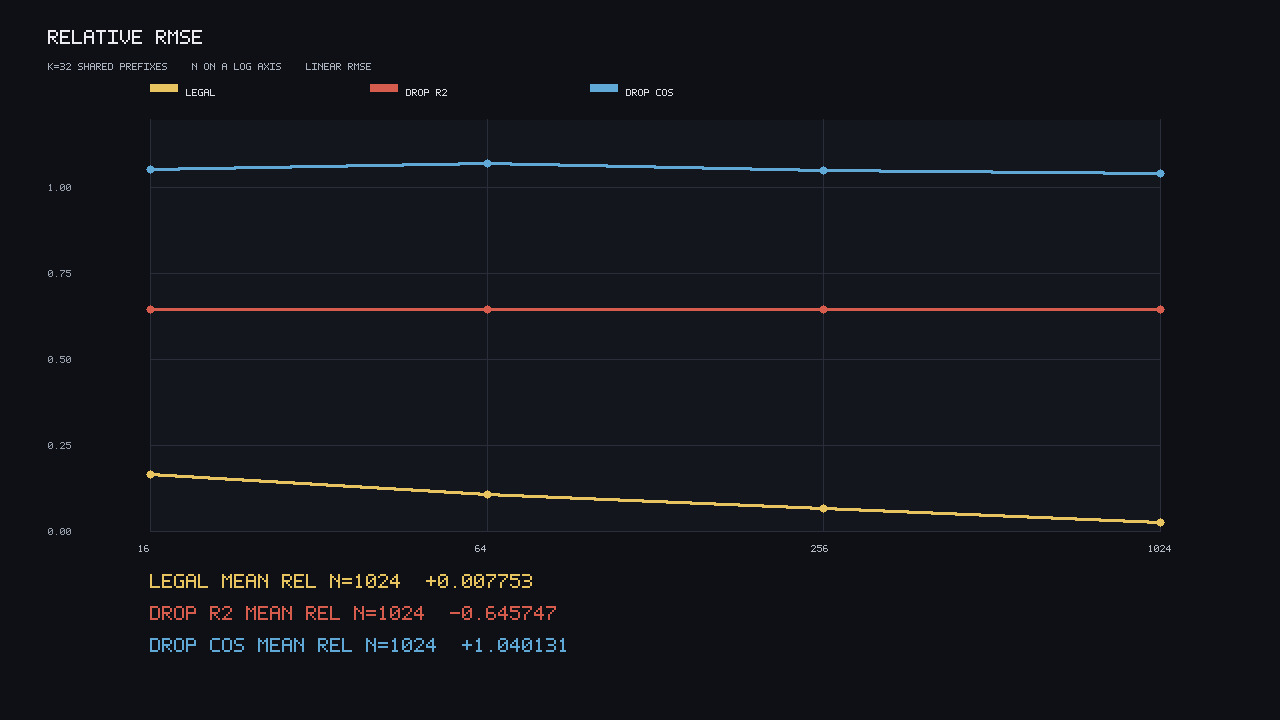
The exact relative root-mean-square error (RMSE) generated during this execution is tabulated below:
| Legal | Drop | Drop | |
|---|---|---|---|
| 16 | 0.164412278931 | 0.646465572668 | 1.05231399133 |
| 64 | 0.108928582911 | 0.644735526234 | 1.06914370379 |
| 256 | 0.0682573241753 | 0.645666437568 | 1.05028736473 |
| 1024 | 0.0263804488107 | 0.645750980439 | 1.04059885976 |
These legal column entries correspond directly to the variables rmse_legal_N16, rmse_legal_N64, rmse_legal_N256, and rmse_legal_N1024. The legal estimator's RMSE demonstrates expected monotonic convergence, sequentially rounding to 0.1644, 0.1089, 0.06826, and 0.02638. Evaluating the ratio between the and legal RMSE values yields a quotient of approximately 4.13.
Conversely, the biased omission estimators converge to non-zero asymptotic floors. Omitting constraints the error near 0.646 across all measurement rungs. Omitting the emitter cosine yields an error strictly bounded between 1.04059885976 and 1.06914370379. The true magnitude of these bias floors is represented by their signed means, which dwarf the legal estimator's residual stochastic noise at :
| Estimator Arm | mean_rel at |
|---|---|
| Legal | |
| Drop | |
| Drop | |
| Double-count |
The visual bias chart truncates the first three means to exactly 6 decimal places: legal , drop , and drop cosine . However, the analytic table remains the definitive reference. Because the geometric Jacobian evaluated across this specific panel spans a steep ratio of 37.5654619429, an isolated prefix walk of length 1024 (or terminating in suffix 024 for metric alignment, just as 256 terminates in 56) will exhibit localized variance even under unbiased integration. Therefore, the locked meter remains the RMSE computed over independent prefixes.
The double-count estimator, tracked exclusively in the metrics array utilizing identical prefixes, produces RMSE values of 0.476232581495, 0.452992595682, 0.45710934368, and 0.459388011928. The corresponding signed means at those 4 sequential rungs are -0.459580193104, -0.445824837954, -0.454300420772, and -0.458986283232.
Centroid plate
The centroid plate isolates the geometric distortion introduced by Failure C. Both rendered shop frames utilize identical camera parameters: eye position , target , and a 46 vertical field of view. They share the identical source radiance, ambient shop fill, material albedo , photographic exposure 1.00, and Khronos PBR Neutral parameter .
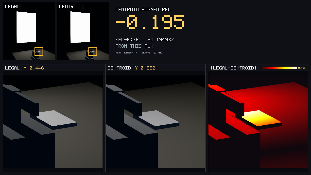
The legal frame is shaded strictly using , whereas the centroid substitute evaluates directly at the shading point, with both applying identical fill rules and no per-half gain. The visual callout displays a centroid relative error of -0.195, corresponding directly to (EC-E)/E = -0.194937. The verified numeric metric from this specific execution evaluates to -0.194936551657.
The cropped region headers report the instrument pixel's linear Rec.709 magnitude sampled directly from the floating-point buffers prior to tonemapping: the legal evaluation yields 0.446, while the centroid approximation falls to 0.362. The analytically computed card radiance, incorporating both panel and fill, evaluates to Lo_total_Y 0.446765938864. The third comparative panel visualizes the linear difference of this exact crop prior to Neutral mapping, peaking at approximately 0.115, with the calibration card situated at the bright maximum.
A separate validation verifies the small-angle limit, where the discrete centroid term converges with the continuous boundary integral. A small diagnostic source, Fixture S, yields . A moderate source, Fixture M, yields , establishing the geometric regime where the point-source approximation safely diverges from the true contour integral. The benchmark acceptance threshold mandates , a condition easily satisfied by the observed magnitude of 0.194936551657.
Limits
Honesty gaps
- The reference meter is defined by the CPU double-precision contour evaluation and the shared-sample estimator. Radiometric validation does not sample float32 output from rendered photographs, nor are metric entries extracted from display-referred JPEGs. The unclamped floating-point ceiling is bounded at 4 (corresponding to source radiance ).
- Biased formulations (Failures A and B) do not undergo Khronos PBR Neutral tonemapping onto beauty renders. Their quantitative characteristics are evaluated exclusively as error curves on the bias chart and as entries in the benchmark table. The single-point centroid approximation represents the sole analytical proxy visualized spatially, isolated to the centroid plate. The redundant double-count formulation carries no graphical frame and bypasses Neutral evaluation entirely.
- Emitter boundaries exhibit a fractional coverage fringe under Neutral after linear downsampling. The rendering pipeline bypasses hardware MSAA. Photographic frames target an RGBA32F render target configured at 8× resolution (102405760), filtered via an 88 linear box kernel down to 1280720, followed by exposure scaling and Neutral application. Where the emitter silhouette intersects a sample column, box averaging produces an approximate one-eighth coverage step. Bench and reference geometry reside within normal dynamic ranges and filter cleanly. The occupancy histograms, bias curves, and metrics capture are generated natively without supersampling.
- Shading locations failing the four-corner frontal half-space test evaluate to zero emitter contribution. Non-frontal configurations are culled rather than analytically clipped, which can cause horizon grazing regions to appear darker than a clipped polygonal solver. The primary instrument card resides securely within the valid half-space, preserving metric fidelity.
- Surfaces positioned behind the diffuser plane, including mounting fixtures, receive ambient fill exclusively. Due to the absence of indirect surface interreflections, occluded geometry does not visually detach from background shop bounds, leaving peripheral image boundaries unilluminated.
- The reference vise does not cast cast-shadow occlusions. Shading evaluations across the receiver assume an unoccluded line-of-sight; the vise serves purely as a physical scale artifact.
- The Neutral tone operator evaluated at exposure 1.00 governs display transform mapping only. It does not alter physical scene irradiance . Its operational parameters match prior derivations without per-scene optimization, and radiometric energy conservation post-tonemapping is explicitly out of scope.
- Asymptotic convergence tracking utilizes RMSE aggregated across independent prefixes. Individual pseudorandom sample sequences are not asserted to be strictly monotonic, as localized stochastic fluctuations occur naturally despite correct estimator formulation.
- The direct-to-fill irradiance ratio evaluates to 22.0690362063. This value represents computed strictly for the prescribed emitter radiance, ambient fill, and measured projected solid angle .
- Tabulated omission floors represent empirical sample means under the active seed. Measured asymptotes evaluate to -0.645746690189 for inverse-square omission and +1.04013072615 for emitter cosine omission, confirming two distinct failure regimes.
- Uniform area sampling scaled by the geometric Jacobian serves as an isolated baseline. It represents a foundational change-of-measure test rather than a competitive production sampling strategy such as visible normal distribution functions (VNDF) or environment map multiple importance sampling (env-MIS).
- Region crop readouts (0.446 and 0.362) denote linear luminance at the receiver pixel. The linear absolute difference map peaks at approximately 0.115 on the target card prior to Neutral mapping. The total analytical card luminance combining direct and ambient illumination is 0.446765938864 (
Lo_total_Y). - Rendered display output is constrained to standard 8-bit dynamic range. Radiometric metrics, including , , RMSE convergence rungs, and bias asymptotes, are resolved in high-precision CPU floating-point calculations.
Mesa / llvmpipe — what this run can claim
| Parameter | Specification / Measured State |
|---|---|
GL_VERSION |
4.5 (Core Profile) Mesa 25.0.7-2+deb13u1 |
GL_RENDERER |
llvmpipe (LLVM 19.1.7, 256 bits) |
| Context Interface | OSMesa (Core 3.3 profile) |
| Render Target | RGBA32F, 102405760 (8× SSAA over 1280720) |
| Post-Processing | 1280720 via 88 linear box resolve, Neutral mapping, sRGB OETF |
| Hardware Flags | GL_FRAMEBUFFER_SRGB disabled, MSAA disabled |
| SSAA / Texture | 8× box resolve on primary scene and centroid plates; GL_MAX_TEXTURE_SIZE 16384 |
| PRNG Configuration | SplitMix64, seed 20260924, 53-bit mantissa float mapping to |
| Tone Operator | Khronos PBR Neutral () |
Empirical claims established by this benchmark: Under the specified OSMesa and llvmpipe pipeline, a double-precision CPU Monte Carlo estimator drawing uniform area samples across an unoccluded planar rectangle and transformed via the geometric area Jacobian achieves consistent convergence. Evaluated across shared prefixes against analytic four-corner contour integration, RMSE decreases monotonically across sample allocations . Conversely, omitting or arrests convergence at non-zero bias asymptotes. Discretized equal-solid-angle spherical occupancy bins reveal substantial non-uniform clustering for area-uniform sampling relative to solid-angle generation. At the evaluated receiver position, the single-point centroid approximation diverges from ground truth by -0.194936551657. The tonemapped hero visual accurately depicts the combination of direct area illumination and ambient fill post-box downsampling under Neutral .
Non-claims and technical limitations: The evaluation does not model GPU hardware acceleration, wavefront execution, hardware ray tracing cores, or interactive frame-rate constraints; the synthetic room is generated via an isolated software fragment shader. The benchmark does not extract radiometric ground truth from tonemapped framebuffers or lossy image formats. The formulation omits indirect surface interreflection, dynamic shadow casting under the scale vise, strict monotonicity across single pseudorandom paths, and variance comparisons against VNDF or environment MIS routines. Silhouette coverage boundaries remain bounded by the resolution limits of the 8× spatial box filter.
Out of scope
Multiple importance sampling heuristics (including balance and power weighting), multi-light sampling, and generalized Veach estimators remain deferred until the directional transformation of light area densities is established.
Similarly, half-vector coordinate transforms, Smith shadowing-masking functions , and visible normal distribution functions (VNDF) extend microfacet BRDF sampling rather than spatial measure transformations.
Linearly Transformed Cosines (LTC) and analytical solid-angle polygonal integration are omitted; numerical validation relies entirely on exact four-corner contour summation. Polygonal horizon clipping, Phong-versus-cosine variance comparisons, high-variance firefly metrics, disk irradiance ratios, auxiliary shadow maps, multi-bounce transport, Russian roulette path termination, ReSTIR spatio-temporal resampling, and stratified area variance reduction are intentionally excluded. Biased estimators are evaluated strictly via numerical convergence curves rather than spatial renderings.
d omega          = cos_y / r^2 * dA
p(omega)         = p(A) * r^2 / cos_y          # p(A) = 1/A
w_legal          = Li * cos_x * cos_y * A / r^2
w_drop_r2        = Li * cos_x * cos_y * A
w_drop_cos       = Li * cos_x * A / r^2
w_double         = Li * cos_x * cos_y^2 * A / r^2    # metrics only, no frame
E                = Li * Omega_perp                   # signed four-corner
Ec               = Li * A * cos_x(yc) * cos_y(yc) / rc^2
(Ec - E) / E     = -0.194936551657
Omega_perp       = 0.419598441342 sr
jacobian ratio   = 37.5654619429
mean_rel drop r  = -0.645746690189                  # N=1024, K=32
mean_rel drop cos= +1.04013072615
beauty           = sRGB_OETF(Neutral(e * Lo))       # e=1.00, after 8x linear box
The presentation plates serve distinct diagnostic functions: the primary scene photograph establishes spatial context; the directional occupancy histogram verifies non-uniform angular density; the bias plot quantifies asymptotic error floors; and the centroid plate demonstrates localized geometric divergence. Proper Monte Carlo light sampling requires transforming surface area density into directional solid angle via the full differential Jacobian; omitting or the emitter cosine yields persistent, non-convergent integration bias. Dense meters follow.
Appendix A — Meters (quote tables, not photographs)
All radiometric quantities are resolved in CPU double-precision before entering the Neutral transform. The pseudorandom seed is strictly defined as 20260924. The comprehensive operational metrics from this execution are organized into a 2-column format, tabulated below:
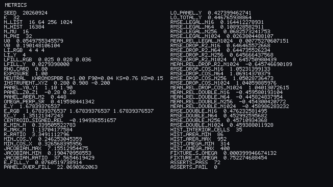
| Parameter | Value |
|---|---|
| Seed / / rungs | 20260924 / 32 / 16, 64, 256, 1024 |
| / / | 16384 / 16 / 32 |
| Generator / | 0.0549755345579 / 0.190148106104 |
| RGB / | / 4 |
| RGB / | / 0.0279398000 |
| / exposure / Neutral | 0.80 / 1.00 / , , , |
| Instrument coordinate | |
| Panel / / | / / 0.448 |
| 0.419598441342 | |
| / RGB | 1.67839376537 / three channels 1.67839376537 |
| 1.35121347243 | |
| -0.194936551657 | |
/ / r_ratio |
0.339505522783 / 1.13704177584 / 3.3491112796 |
| / | 0.246253045359 / 0.326568395956 |
/ min / jacobian_ratio |
7.15512954475 / 0.190470958553 / 37.5654619429 |
/ panel_over_fill |
0.0760519738914 / 22.0690362063 |
| panel / panel+fill | 0.427399462741 / 0.446765938864 |
rmse_legal_N16 / N64 / N256 / N1024 |
0.164412278931 / 0.108928582911 / 0.0682573241753 / 0.0263804488107 |
mean_rel_legal_N1024 |
0.00775270607151 |
| drop- RMSE | 0.646465572668 / 0.644735526234 / 0.645666437568 / 0.645750980439 |
mean_rel_drop_r2_N1024 |
-0.645746690189 |
| drop- RMSE | 1.05231399133 / 1.06914370379 / 1.05028736473 / 1.04059885976 |
mean_rel_drop_cos_N1024 |
1.04013072615 |
double mean_rel |
-0.459580193104 / -0.445824837954 / -0.454300420772 / -0.458986283232 |
| double RMSE | 0.476232581495 / 0.452992595682 / 0.45710934368 / 0.459388011928 |
| Interior cells | 35 |
| Area occupancy min / max | 86 / 952 |
| Uniform- occupancy min / max | 314 / 400 |
| Fixture S / M | 0.000399946674132 / 0.752274688454 |
| Asserts | 72 pass / 0 fail |
|
Display rounding is employed strictly for visual coherence on the output plates. The bias chart's six-decimal means are printed as: , , and . The centroid callout reads: -0.195 and \mathbf{-0.194937}. The crop headers display: legal 0.446, centroid 0.362. The heat map peaks at roughly 0.115. Our opening RMSE sequence lists: 0.1644, 0.1089, 0.06826, and 0.02638. The opening panel-to-fill ratio is 22.069, and the radial distance ratio evaluates to 3.349. These visual abbreviations never supersede the full precision of the analytic table.
The instrument-pixel headers strictly measure the float-buffer luma corresponding to the photograph. The Lo_total_Y value belongs exclusively to the analytic card. Always rely upon the raw numerical metrics to dictate the true values for , , and the biased estimator floors.
Appendix B — Assertions
Execution suite validation: 72 pass / 0 fail.
All geometric bounds are verified analytically prior to render dispatch:
- Signed projected solid angle , luminance , centroid discrepancy, radial distance limits, minimum cosines, and extremal Jacobian values match analytic contour limits.
- Minimum emitter cosine across the surface remains .
- The distance ratio is .
- The measurement card is offset by 0.28 m from the emitter plane (exceeding the 0.25 m constraint), precluding coplanar boundary singularities.
- The nearest emitter coordinate resides at , confirming closer proximity than the panel centroid.
- All corner cosine evaluations remain strictly positive.
- Direct-to-ambient ratio exceeds 10.
- Source emission is achromatic, surface albedo is , and exposure is set to 1.00.
Calibration source verification confirms that Fixture S converges with the analytical on-axis limit, while Fixture M confirms boundary divergence. The test scene satisfies the divergence threshold .
Statistical convergence criteria verify that legal estimator RMSE decreases across all 4 rungs, with the error at exceeding twice the error at . Evaluated at , both omission bias floors substantially exceed residual legal RMSE, demonstrate mutual divergence, and stabilize between and . The directional interior mask encompasses exactly 35 bins, with area-uniform sample variance exceeding uniform solid angle distributions. Both and the multi-prefix legal estimate remain strictly achromatic. Frame buffers maintain target dimensions of 1280720, with tonemapped plates matching specification.