Journal

animated explainers · rendering · sampling

The Half-Vector Jacobian — Visible Normals of Isotropic GGX

Frank Yin
· 6:12
Share

An animated walkthrough of why rough metal turns noisy at grazing angles, and how sampling only the microfacet normals the viewer can see fixes it.

#graphics #sampling

Appendix / Measurements full write-up, figures and tables

Abstract

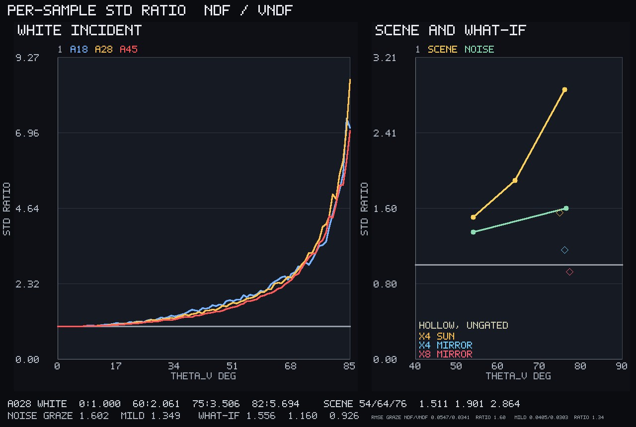
Rough metal seen at a grazing angle, like sunset glare on a wet road or a metal floor under a low camera, is where a path tracer struggles most. Drawing microfacet normals from the GGX distribution wastes many samples on facets the viewer cannot see, and the samples that survive carry weights with no upper bound. This video builds the fix step by step: the half-vector Jacobian, the distribution of visible normals, and the spherical-cap construction of Dupuy and Benyoub that samples it. On a galvanized steel sluice gate at α=0.28\alpha=0.28, visible-normal sampling removes the back-facing draws (27.9% of naive draws at 82∘82^\circ) and lowers the per-sample standard deviation by 3.5× at 75∘75^\circ and 5.7× at 82∘82^\circ. In the ray-traced scene the gain shrinks to 1.6×, and with an 8× sun on the mirror direction it reverses slightly (0.926×), which is the case light sampling with multiple importance sampling is built for.

Key figures
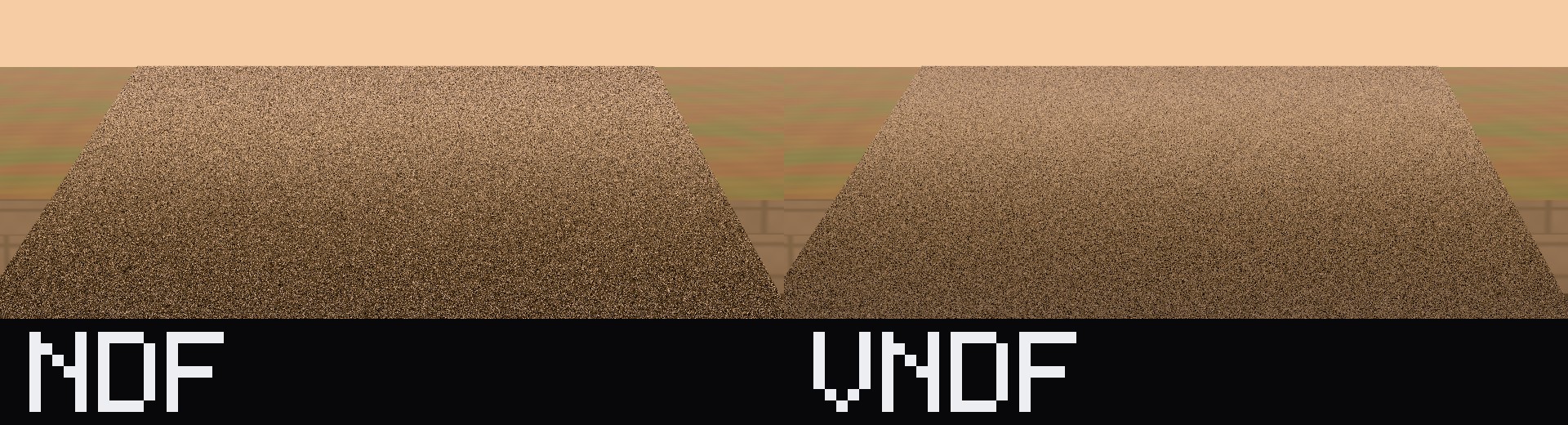
Far end of the sluice leaf at 32 samples per pixel, same seed. Left: sampling the distribution of normals. Right: sampling visible normals.

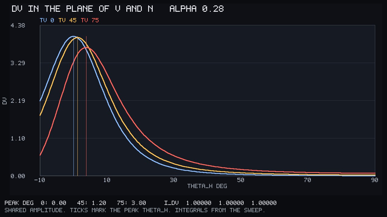
The visible-normal distribution in the plane of view and normal, alpha 0.28, at view angles 0, 45 and 75 degrees.

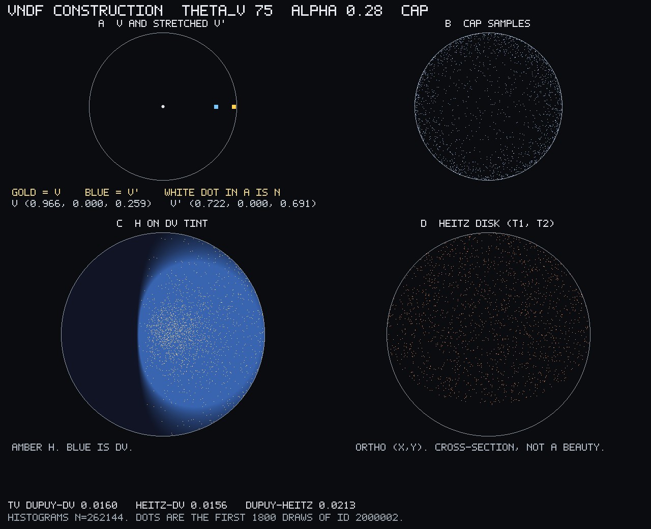
The spherical-cap construction at a 75 degree view, alpha 0.28, with Heitz's projected-disk sampler as the control.

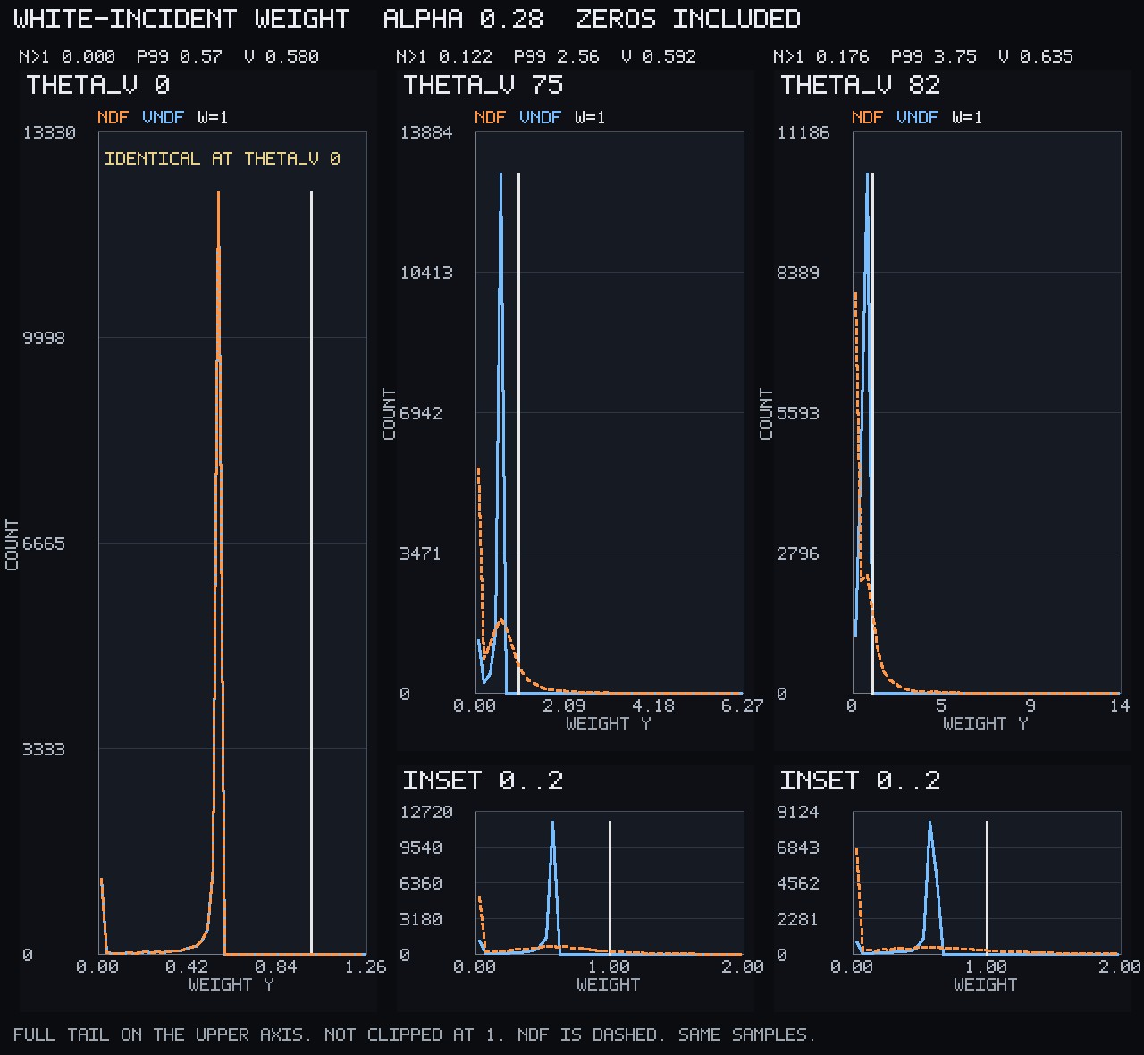
Sample-weight histograms at view angles 0, 75 and 82 degrees. The naive weight has a long tail past 1; the visible-normal weight stays below 1.

Per-sample standard-deviation ratio, naive over visible-normal sampling, against view angle, with the ray-traced scene and the bright-sun cases.

References

  • E. Heitz. Sampling the GGX Distribution of Visible Normals. Journal of Computer Graphics Techniques 7(4), 2018.
  • J. Dupuy, A. Benyoub. Sampling Visible GGX Normals with Spherical Caps. Computer Graphics Forum 42(8), 2023.
  • B. Walter, S. R. Marschner, H. Li, K. E. Torrance. Microfacet Models for Refraction through Rough Surfaces. Eurographics Symposium on Rendering, 2007.