Journal

阴影贴图偏移作为几何误差

Shadow-map bias represents a physical length along the light ray, added just before the depth comparison. Applying too little of this length causes an analytically lit receiver to be incorrectly classified as shadowed, resulting in acne. Applying too much detaches the contact shadow of a thin occluder from its true foot, creating peter-panning. The overarching curve in this note visualizes the exact trade-off between these two artifacts.

Topics such as discrete depth encoding, winner-islands, and reverse-Z belong to the previous note, Z-fighting is geometric compression plus quantization. That text already refers here for the distinction between acne and peter-panning, and fight-fractions remain in that scope. This note fixes a single shadow map and avoids sweeping a depth code. The shared underlying concept is strictly geometric: a depth failure can be quantified as a physical length. There, it is a resolvable interval in front of the camera; here, it is a bias $b$, measured in metres along the sun ray.

The test scene is a service-yard curb. An asphalt apron, a 160 mm concrete curb, a poured wash ramp pitched at $20^\circ$, and a 12 mm steel plate are arranged in a single $1280\times 720$ frame. The lighting environment consists of one directional sun at an altitude of $32^\circ$, casting into a single $512^2$ depth-compare map with an 8 m orthographic projection. The shadow map is rendered exactly once. Across the evaluated ladder, only the compare bias changes.

The beauty pass uses Mesa llvmpipe in scene-referred linear Rec.709, followed by the display path detailed in Tone Mapping: Scene-Referred to Display-Referred. We apply Khronos PBR Neutral using parameters $e=\mathbf{1.00}$, $F_{90}=0.04$, $K_s=0.76$, and $K_d=0.15$, finishing with the sRGB OETF evaluated on the CPU. The exposure gain is locked at $K=\mathbf{3.40}$ for all bias samples. Neutral merely assigns display codes; it has no influence on the acne fraction or the contact gap.

The optimization curve selects the operating point $b^\star=\mathbf{36}\,\mathrm{mm}$ ($0.036\,\mathrm{m}$). As the bias increases from $b=0$ through $b^\star$ to $b_{\max}=120\,\mathrm{mm}$, ramp acne $A_{\mathrm{ramp}}$ falls from $0.509$ through $0.019$ to $0$, and apron acne $A_{\mathrm{apron}}$ drops from $0.483$ to $0$. Conversely, the contact gap $G$ widens from $0$ through $15\,\mathrm{mm}$ to $91\,\mathrm{mm}$. Relying instead on slope-scale at $k_s=1$ and $b_c=0$ clears both acne fractions while maintaining a gap of just $13\,\mathrm{mm}$. By comparison, the smallest constant sample with identically resolved ramp acne sits at $b_{\mathrm{match}}=40\,\mathrm{mm}$, where the gap has already stretched to $20\,\mathrm{mm}$. The verification suite prints 11 pass / 0 fail.

These abbreviated figures map onto the unrounded tokens of this run as follows:

What you are seeing

The visual working space for the scene photographs is scene-referred linear Rec.709, processed through Khronos PBR Neutral at $K=3.40$ and $e=1.00$. In contrast, the sweep plot and the metrics snapshot are authored natively in sRGB and bypass the Neutral mapper entirely. The records are intentionally separated: the photographs illustrate the physical curb, while the tables explicitly quantify $A$ and $G$.

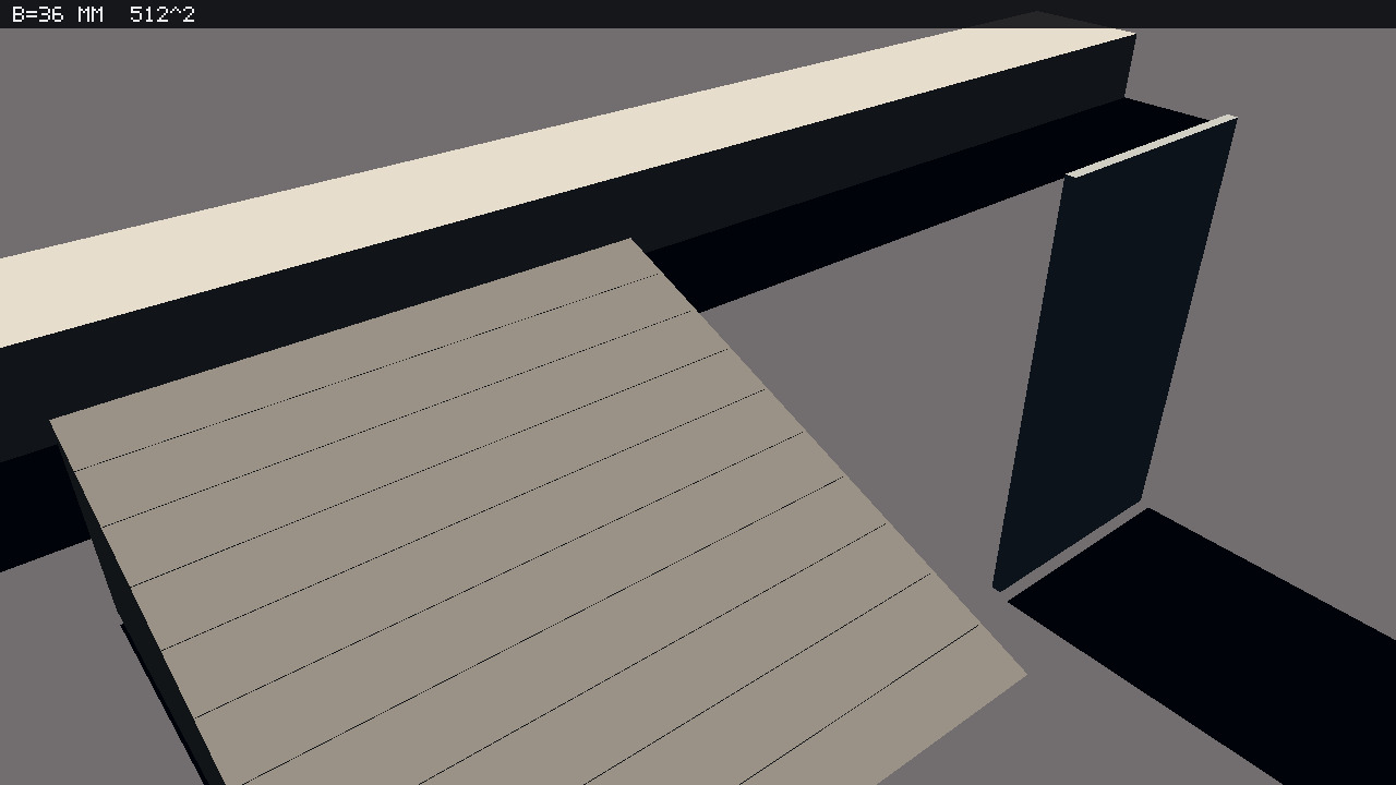
Cover — the operating point. Captured at $1280\times 720$ with a bias of $b^\star=36\,\mathrm{mm}$, showing the service-yard curb, wash ramp, and steel plate. The on-screen HUD displays a single line containing the bias and the $512^2$ resolution. A faint shadow residue remains visible on the ramp, while the apron reads completely clear. This residue corresponds to the leftover ramp acne of $0.018868$ recorded in the table, whereas the clear apron reflects an $A_{\mathrm{apron}}=0$ at this sample. The $15\,\mathrm{mm}$ gap denotes a physical length across the apron, rather than a mere grey level in the JPEG.

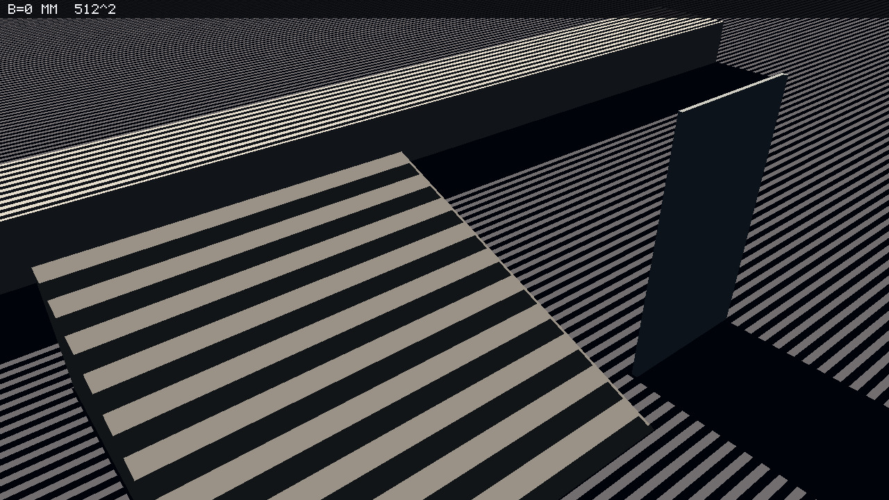
Acne — the short end. This frame shares the same camera and shadow map, evaluated at $b=0$. Both the ramp and the apron incorrectly self-shadow in prominent stripes. Each stripe represents a receiver with an analytic visibility of 1 that the comparison logic has erroneously marked as shadowed. Here, the ramp acne peaks at $0.509434$ and the apron acne reaches $0.482759$, keeping the contact gap tightly at $0$.

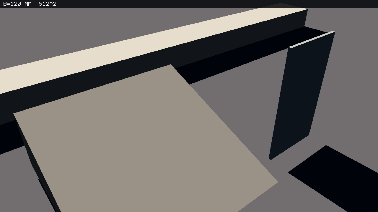
Peter-panning — the long end. Captured with the same camera and map at $b=b_{\max}=120\,\mathrm{mm}$. At this extreme, both acne fractions have successfully fallen to $0$. However, the plate’s contact shadow has visibly detached from its foot. The measured gap along the apron now spans $91\,\mathrm{mm}$ ($0.091\,\mathrm{m}$). The pronounced dark band highlights this detachment, while the curb’s inherent occlusion remains a distinct, separate shadow.

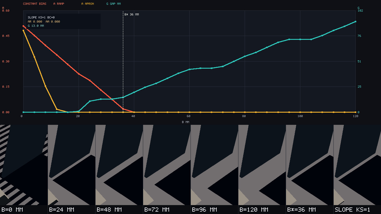
Sweep — teaching pin. This plot graphs $A_{\mathrm{ramp}}$, $A_{\mathrm{apron}}$, and $G$ against a constant bias, marking $b^\star$ explicitly alongside the slope-scale triple as a special callout. Eight specific contact strips sit underneath the main plot: the samples nearest $0$, $24$, $48$, $72$, $96$, and $120\,\mathrm{mm}$, followed by $b^\star$, and finally the slope-scale result. The quantised staircase nature of $G$ is left visible to accurately reflect the data. This figure visually summarizes the trade-off. The subsequent table highlights selected rows from this sweep; the plot supplements rather than replaces the raw numbers.

The table below extracts selected constant-bias samples from this run. The full evaluation ladder consists of 31 samples ranging as $b=0,4,\ldots,120\,\mathrm{mm}$, which are all plotted on the preceding figure.

At $b=0$, the contact gap remains strictly closed, but approximately half of each lit grid registers as false shadow. Apron acne is fully resolved by $16\,\mathrm{mm}$, though the ramp still exhibits an acne fraction of $0.283019$ while the gap remains closed. Progressing to $b^\star$, the ramp fraction diminishes to $0.018868$, the apron is entirely clear, and the gap has just begun to open to $15\,\mathrm{mm}$. The ramp fraction finally reaches zero at $40\,\mathrm{mm}$, incurring a gap of $20\,\mathrm{mm}$. Pushed to the extreme at $120\,\mathrm{mm}$, both acne fractions are zero, but the gap expands unacceptably to $91\,\mathrm{mm}$. The chosen operating point sits strategically in the interior space where ramp acne is largely suppressed and the contact gap has only just started to pull away.

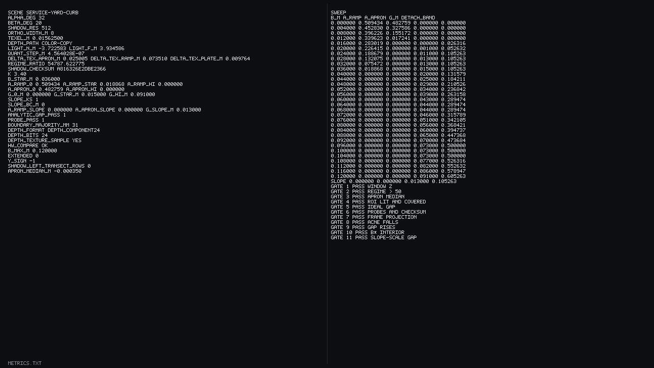
Metrics snapshot. A captured image of this run’s parameter table. Should any glyph appear soft or clipped in the image, the text-based markdown tables serve as the definitive reference.

Bias as a length on one map

The shadow map stores a single depth value per texel, representing the front-most surface rasterized from the light's perspective. The subsequent depth comparison simply asks whether the shaded point sits farther from the light than this stored depth. For surfaces that tilt across the texel, the majority of shaded points naturally fall farther away than the front-most fragment, causing them to fail the comparison. Acne is the direct visual manifestation of this mismatch: the receiver’s analytic visibility toward the sun is 1, yet the depth compare incorrectly classifies it as shadowed.

Given this specific frustum, the texel slope heavily dominates the 24-bit quantisation step. The geometric slope across the apron spans $0.025005\,\mathrm{m}$ per texel, while the depth quantisation step is a mere $4.564028\times 10^{-7}\,\mathrm{m}$. The ratio between them is $54787.622775$ (roughly $54788$), which easily clears the acceptance gate threshold set at $50$. Consequently, the acne observed in the cover’s family of frames is strictly a texel-slope failure. Phenomena such as winner-islands are categorized differently and remain detailed in the z-fighting note.

Introducing a bias $b$ subtracts a physical length along the ray just prior to the depth comparison, effectively pushing the shaded point toward the light source. A sufficiently large $b$ absorbs the texel mismatch, causing the acne fraction to reliably fall. However, this identical spatial push shifts the shadow boundary of any thin occluder away from its true physical contact point. The stretch of ground between the physical foot and the displaced shadow boundary is analytically shadowed, but the depth compare incorrectly evaluates it as lit. This detached length, when measured along the apron, is precisely the contact gap $G$.

The presence of two distinct receivers prevents this trade-off from collapsing into a single, trivial slope. The wash ramp is lightly grazed by the sun at a shallow incidence of $12^\circ$. Conversely, the apron faces the sun more directly, determined by the sun’s unadjusted altitude of $32^\circ$. A constant bias large enough to quiet the severe acne on the ramp immediately induces a visibly detached gap at the steel plate. A slope-scale approach, however, adaptively applies a larger offset for the ramp’s steep texel slope and a comparatively shorter length for the apron. This intelligent scaling forces the marked point off the traditional constant-bias curve, driving ramp acne down while maintaining a tightly controlled gap.

The sample at $b=0$ anchors the acne-heavy end of the spectrum, whereas $b=b_{\max}=0.120\,\mathrm{m}$ anchors the peter-panning end. The cover image represents the balanced interior sample, $b^\star$. Crucially, all three configurations share the exact same camera, exposure parameters, physical materials, and underlying shadow map. The slope-scale point is highlighted as a distinct callout, appears as the final strip on the teaching figure, and occupies a dedicated row in the metrics table. It serves as a single, highly optimized marked point residing on the exact same theoretical trade-off space.

The compare

The coordinate system is right-handed, with $Y$ designated as up, measured in metres.

A single light camera is utilized across the entire ladder. Depth increases linearly along the $-s$ vector. The orthographic projection uses a square frustum with a width of $W_l=8\,\mathrm{m}$. Window depth is defined as:

For this run, the near and far planes are set to $n_l=-3.722583\,\mathrm{m}$ and $f_l=3.934586\,\mathrm{m}$, respectively, resulting in a world-space texel size of $t=0.015625\,\mathrm{m}$ ($15.625\,\mathrm{mm}$). The corresponding quantisation step is $4.564028\times 10^{-7}\,\mathrm{m}$. Calculated texel slopes are $0.025005\,\mathrm{m}$ on the apron, $0.073510\,\mathrm{m}$ on the ramp, and $0.009764\,\mathrm{m}$ along the plate face.

Both the CPU metric analysis and the beauty shader rely on the identical depth compare function. The value $\tilde d$ represents the stored window $z$ of the winning fragment, subsequently decoded using the identical $n_l$ and $f_l$ parameters. The depth fetch relies strictly on point sampling (nearest texel). The bias function $b(n_p)$ is evaluated directly against the receiver's geometric normal.

Constant sweep. For the baseline evaluation, $k_s=0$, reducing the bias function to $b(n)=b$. The measurement ladder spans $b=0,4,\ldots,120\,\mathrm{mm}$, yielding a total of thirty-one distinct samples. The underlying shadow map is rendered only once. The map's cryptographic checksum, a816326e2dbe2366, remains perfectly stable across every evaluated $b$, including after the final beauty frame has finished rendering. The applied bias exists strictly within the comparison operator, never modifying the stored depth.

Slope-scale, one marked point. For this focused test, the constant bias is dropped ($b_c=0$) and slope-scaling is enabled ($k_s=1$). On a planar surface, defining $e_1$ and $e_2$ as the axes of the light image, we have:

Because these derivatives are calculated per metre in the light image, $\Delta_{\mathrm{tex}}$ effectively describes the metres of light depth traversed across a single shadow texel. On the flat, un-averaged geometry, this calculated length directly dictates the bias: $73.510\,\mathrm{mm}$ across the ramp and $25.005\,\mathrm{mm}$ across the apron. Note that the Khronos Neutral shoulder constant $K_s=0.76$ is purely a display-space parameter and represents a completely different symbol from this slope multiplier $k_s$.

Acne fraction. This metric evaluates a receiver region subdivided into a strict $8\,\mathrm{mm}$ grid. A grid sample is only considered if its analytic visibility toward the directional sun evaluates exactly to 1.

Both the ramp and apron evaluation grids adhere strictly to this definition. In this specific scene configuration, both regions are entirely analytically lit: the ramp verifies at $2703/2703$ samples, and the apron at $3654/3654$.

Contact gap. The downstream face of the steel plate rests at $x_c=1$, presenting a material thickness of $\tau=12\,\mathrm{mm}$ facing the sun. When analyzing the raster map, each visible ground segment is majority-filtered using a $31\,\mathrm{mm}$ sliding window; this filter is strictly isolated to finding the shadow boundary. The gap metric $G$ is defined as the starting coordinate of the longest continuous shadowed run, minus the physical edge coordinate $x_c$. Crucially, this spatial filter is never applied to the acne metric $A$. Immediately downstream of the plate, evaluated at $b=0$, the raw comparison algorithm correctly shadows $451/451$ measured transect samples. This confirms that the fully closed gap is a genuine physical contact shadow, rather than an artifact of a missing shadow caster.

Ideal-map oracle. We employ a continuous analytical model as a unit test for the raster metric, scoped specifically for this plate and sun altitude:

The response curve features a distinct knee precisely at $b=\tau/\cos\alpha$. When executed as an unfiltered walk across the ideal continuous depth profile, the algorithm aligns with $G_{\mathrm{ideal}}$ to within $1.5\,\mathrm{mm}$ across all five locked biases. The highest recorded walk error peaks at only $0.647\,\mathrm{mm}$. Note that the measured raster gap is empirically sampled and is not artificially fit to this oracle.

Operating point. By normalizing against the baseline extremes—defining $A_0=A_{\mathrm{ramp}}(0)$ and $G_{\mathrm{hi}}=\max(G(b_{\max}),0)$—we construct an objective function:

The optimal bias is computed as $b^\star=\arg\min J$, where any tie defaults to the smaller $b$. For this particular run, the solver identifies the global minimum at $b^\star=36\,\mathrm{mm}$ yielding a score of $J=0.202$, which lands cleanly in the interior between the two swept extremes. The sample sweep was deliberately not extended beyond this bound.

Slope-scale as one marked point

Slope-scale represents a highly optimized point within the same conceptual trade-off space, defined by $k_s=1$ and $b_c=0$, where spatial derivatives are computed in shadow-texel units. During this run, that specific configuration successfully clears both acne fractions (achieving $A_{\mathrm{ramp}}=0$ and $A_{\mathrm{apron}}=0$) while holding the contact gap tightly at $13\,\mathrm{mm}$ ($0.013\,\mathrm{m}$).

Quote the metrics. The photographs are not the meter.

The metrics are evaluated in double-precision on the CPU, strictly before the Neutral tone mapper is applied. The beauty display utilizes Khronos PBR Neutral at $e=1.00$, employing the static constants established in the tone-mapping note rather than re-fitting them per bias sample.

Honesty

1. The meter relies on the CPU compare. It evaluates the float color copy of the winning fragment depth against the analytic visibility grids. Both the acne fractions and the gap are derived strictly from this comparison. The shading probes sample world points using the beauty compare logic. At both $b=0$ and $b^\star$, the bits match the CPU function precisely, recording $16/16$.

2. Gate 3, the apron median. The measured apron median of $d-\tilde d$ is $-0.000350\,\mathrm{m}$ ($-0.35\,\mathrm{mm}$). This sits a third of a millimetre below the strict planning floor of 0, arising because the 8 mm evaluation lattice rests slightly sunward of the $512^2$ texel centers. Evaluating the same grid directly against those texel-center depths predicts $-0.349\,\mathrm{mm}$. The control safely accepts medians above $-2\,\mathrm{mm}$. By comparison, an undrawn apron would land near $-3.3\,\mathrm{m}$.

3. Neutral may shoulder the plate’s lit face. Specular highlights on the plate are structurally gated by the shadow bit and do not factor into $A$ or $G$. The final display energy after the Neutral pass is not a subject of this claim. The exposure $K=3.40$ is held fixed rather than retuned per bias, utilizing the established constants from the tone-mapping note.

4. $G$ is a staircase. The $31\,\mathrm{mm}$ majority window is employed exclusively to locate the contact boundary and is never applied to the acne calculation. The shipping gate formally demands only that $G(b_{\max})>G(0)$. Adjacent samples along the sweep are permitted to step backward. However, on this specific run, the series does not regress: it holds on flat landings before rising monotonically from $0$ to $0.091\,\mathrm{m}$.

5. Slope-scale is one marked point. The specific claim is that $G(k_s=1)<G(b_{\mathrm{match}})$ at matched ramp acne. Percentage-closer filtering, variance and exponential shadow maps, and cascades are outside this measurement.

6. One map, one checksum. The shadow pass runs once. A checksum mismatch stops the run. This run’s checksum a816326e2dbe2366 is constant across the sweep and after the last beauty.

7. Rasterization is llvmpipe’s. The ideal-map oracle checks the metric code. The raster curve checks the shadow map. There is no discrete-GPU depth claim, no hierarchical-Z claim, and no vendor polygon-offset scale.

This run can claim the following. On this OSMesa / llvmpipe build, one directional sun, one $512^2$ nearest-texel shadow map, and one constant-bias sweep from 0 to 120 mm produced a falling acne fraction on both receivers and a rising contact gap at a 12 mm plate. The operating point that minimises the normalised sum of ramp acne and gap is the interior sample $b^\star=36\,\mathrm{mm}$ ($J=0.202$). Slope-scale at $k_s=1$ clears ramp acne at a shorter gap than the matching constant sample, 13 mm against 20 mm. The regime ratio places the failure in the texel-slope regime. The run prints 11 pass / 0 fail.

This run does not claim the following. A GPU, a wavefront, or a frame-time budget. A filtered shadow, a cascade, or a soft penumbra. A measured polygon offset, a normal-offset bias, or a receiver-plane depth. Acne or gap read from a JPEG. A second depth codebook, a fight-fraction, or a reverse-Z curve. A ranking of this bias length against a product shadow stack.

The eleven checks cover window depth, the regime ratio, the apron median, lit and covered regions, the ideal-map gap, probes and the checksum, frame projection, falling acne, a rising gap, an interior operating point, and the slope-scale gap.

Percentage-closer and contact-hardening filters, cascades, and atlas packing sit outside the measurement, as do a second light, an animated sun, and a soft penumbra. So do reverse-Z, a depth-format sweep, and the z-fighting note’s fight-fractions. The cover is the operating point. The sweep is the teaching figure. Bias is a geometric length, and the curve is the photograph.