
Our previous note addressed a common Monte Carlo sampling mismatch: evaluating the same integral using two different probability density functions at a single sample count, . Those pdfs were properly defined as densities measured in . Because split-sum approximations fold an environment into a GGX prefilter multiplied by a DFG LUT, they leave the measure implicit inside the integral (yielding an environment solid-angle mean luma of 1.628 on that specific loft run). This note focuses directly on formalizing that measure.
Path tracers inherently sample . Irradiance and the rendering equation, however, track the projected solid angle, . A direction is simply a point on the hemisphere, weighted in steradians. Flux passing through a flat surface depends on this projected solid angle, defined mathematically as . Relying on source area, pixel counts, or manipulating as an arbitrary brightness scalar are fundamentally incorrect approaches.
The core of our importance-sampling discussion evaluated a finite disk with an angular radius of 3.600°. The exact solid angle subtended by that disk—which the previous note omitted—is:
Evaluating a full-hemisphere pdf against a spherical cap this small demonstrates exactly why a cosine sample produces fireflies in a highlight. The detailed cosine-versus-Phong comparison remains in that earlier note.
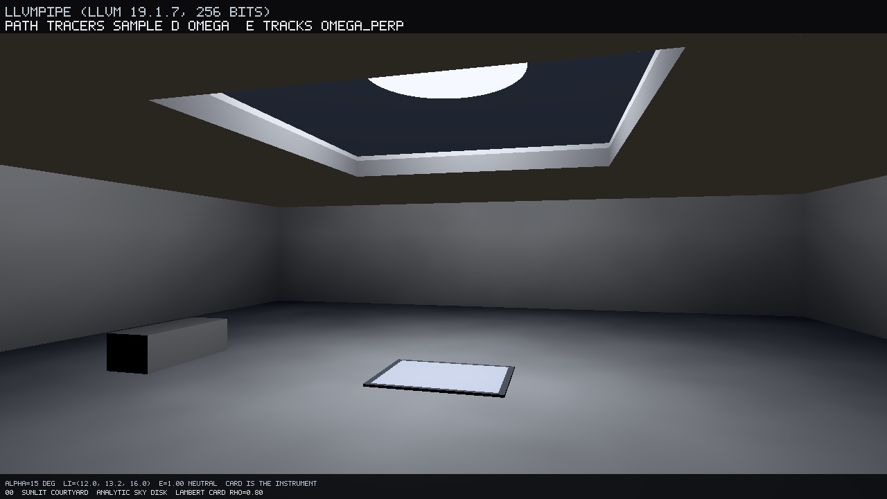
We introduce a new photographic family for this analysis: a sunlit courtyard and skylight atrium. This setup trades the dark oak and lacquer of previous scenes for four walls, a square skylight with a visible jamb, a matte limewash floor, and a single low bench for scale. An analytic sky disk sits in the opening—a spherical cap with a locked half-angle of and uniform radiance. On the floor below rests our primary instrument: a white Lambertian card (, normal , emission ). While the HUD accurately states path tracers sample d omega E tracks Omega_perp, do not attempt to derive visually from this photograph.
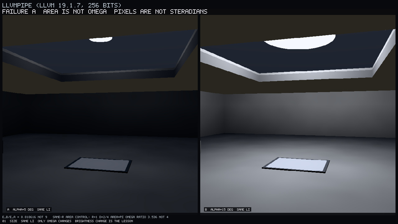
This is the core visual reference. Both shots share the exact same camera, exposure, and incident radiance . The left side features , while the right uses . The right-hand card is visibly brighter because it integrates over more steradians. As the lower caption indicates, only changes; this brightness difference is the primary lesson. It yields an exact irradiance ratio of under our same- control. The fundamental takeaway: area is not , and pixels are not steradians.
Evaluating the system on Mesa 25.0.7 llvmpipe (linear Rec.709, Khronos PBR Neutral with , seed 1352782172), we extract the ground-truth solid angles and irradiance metrics. The naive small-angle approximation of is strictly rejected; under a same- area control, the true ratio is 3.536 (rather than 4). A suite of 28 pass / 0 fail assertions confirms these bounds against the test harness.
| Setup | Solid Angle () | Projected () | Irradiance () Ratio |
|---|---|---|---|
| Cap A () | 0.023909417 sr | 0.023863926 sr | Base |
| Cap B () | 0.214094348 sr | 0.210446804 sr | |
| Ratio (B/A) | 8.954394 | - | - |
The incident radiance remains bit-identical between setups, producing a luminance and a disk-to-fill -ratio of 200.
Scene
Our working color space is scene-referred linear Rec.709. The environment consists of one courtyard, one analytic cap, and one Lambertian card. Display parameters are inherited from previous work: the Khronos PBR Neutral operator evaluated at , followed by the IEC 61966-2-1 sRGB OETF applied on the CPU. We emphasize that the tone curve does not create lighting, and the Neutral operator does not author irradiance (). We refer readers to the tone-mapping and split-sum IBL notes for full display-pipeline context.
Hero — presentation hook. The atrium features the visible disk, white card, and low bench at . This plate establishes the aesthetic baseline, but the final JPEG artifacts are not the measurement tool.
Size A/B — teaching pin. Comparing setups A and B, we maintain the exact same and shared exposure across versus . Precision analysis must rely on the tabular metrics rather than visual perception.
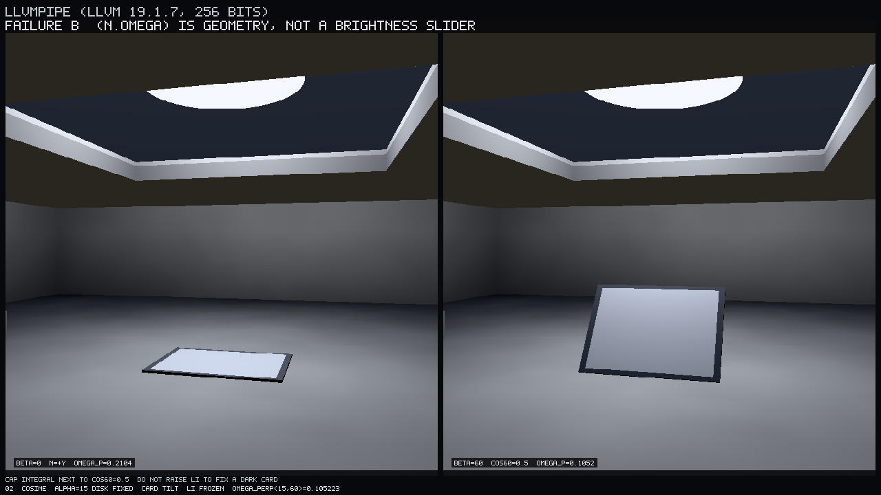
Cosine tilt — Failure B. The disk remains fixed in world space. On the left, the Lambertian card is flat (, ). On the right, the card is tilted to while incident radiance remains frozen. The geometric projection strictly governs this behavior; it cannot be treated as an artistic brightness slider.
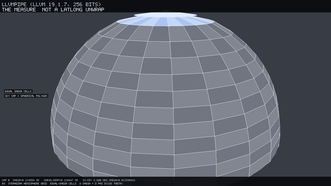
Grid — the measure. A unit hemisphere is projected over the card and discretized into equal- cells. The sky cap is treated geometrically as a spherical polygon. This visualizes the true solid angle measure, avoiding the distortions of a lat-long unwrap.
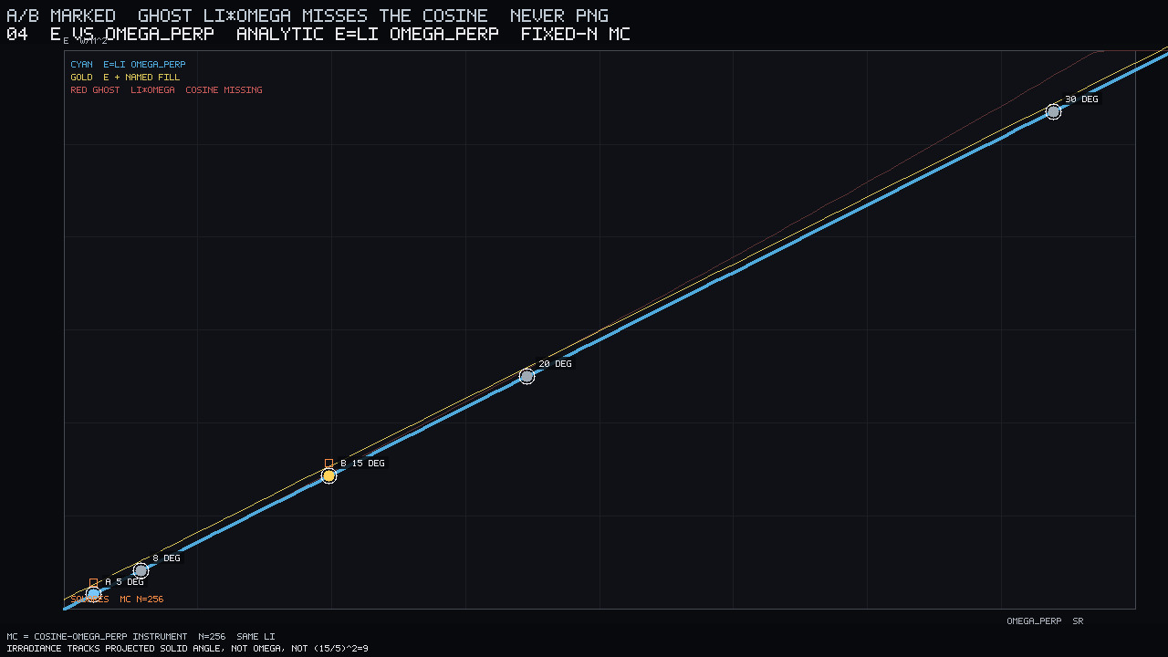
vs — the identity. The horizontal axis tracks in steradians. The cyan line plots the analytic disk irradiance , while the gold line includes the disk alongside named ambient fill. The red ghost trace plots , visually demonstrating the resulting error when the cosine term is incorrectly omitted. The square markers plot our cosine-arm estimator at , inverted through the Lambertian BRDF. The core mathematical identity is upheld: irradiance directly tracks projected solid angle.
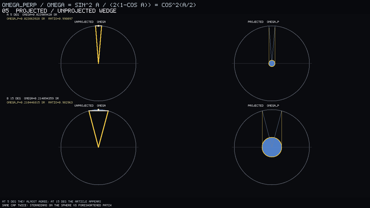
Wedge — the article. We view the same spherical cap twice in profile. The left side visualizes steradians mapped on the unit sphere, whereas the right side shows the foreshortened patch. At a narrow , the two measures nearly agree; at , the mathematical divergence becomes highly pronounced.
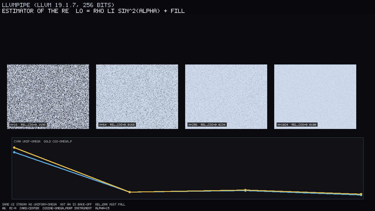
MC- — estimator of that integral. Sampled at the card center using , we evaluate the rendering equation at , , , and samples. The thumbnails depict the cosine- instrument. The plot tracks both uniform- (cyan) and cosine- (gold) integration using the same random stream. This is not an importance-sampling performance comparison; the requirement is that rel_err reliably converges. Traces may oscillate at , but strict error reduction is gated at .
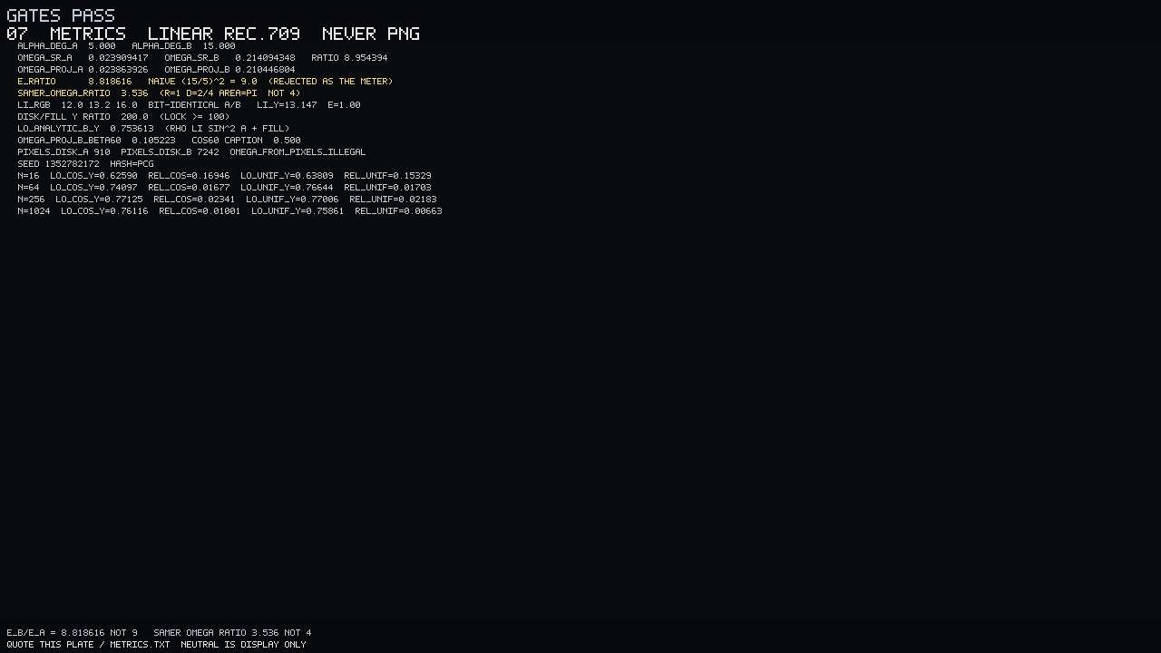
Metrics strip — the meter snapshot. This is the science plate capturing the float-buffer measurements. Data must be quoted from the text table, not inferred from the JPEG.
Maintain a strict separation between these two artifact categories:
- Beauty plates (
00,01,02) represent the GLSL courtyard running on llvmpipe, mapped through Neutral and an sRGB OETF. The shader properly evaluates walls, floor, and the card using a disk form factor. Do not attempt to reverse-engineer , , or from these JPEGs. - Instruments (
03,04,05,06,07, and the metrics block) represent exact float identities and the CPU estimator.
Method
The Rendering Equation Once
We formally state the integral and define all notation. Subsequent derivations rely upon this specific formulation.
| Symbol | Definition | Units |
|---|---|---|
| Outgoing radiance | (linear Rec.709 RGB) | |
| Emitted radiance | ; 0 on the card and floor | |
| Incident radiance | ; piecewise-constant sky disk + fill | |
| BSDF | ; Lambertian | |
| Geometric unit normal | Dimensionless | |
| Incident direction vector | Unit vector, | |
| Outgoing direction vector | Unit vector | |
| Hemisphere about | ||
| Solid-angle measure |
A Monte Carlo path tracer evaluates this integral by drawing samples and computing the estimator . While the implementation of such a tracer is beyond the scope of this note, we strictly focus on validating the radiometric measure represented by .
, Then Projected Solid Angle
Let denote the polar angle measured from the normal , and the azimuthal angle in the local tangent frame.
Grid visualization exploits this latter differential form: uniform intervals in and subtend equal solid angles. To maintain a constant , the necessary polar interval is . Consequently, uniform sampling partitions are broad near the pole and dense near the horizon. Thus, a latitude-longitude parameterization that is uniform in produces visually isotropic texture cells but highly distorted elements that scale proportionally with . Drawing uniform across necessitates generating samples via the inverse cumulative distribution functions and .
Integration over the full sphere yields , and over the hemisphere . In our test framework, sphere_sr returns 12.566370614 and hemisphere_sr returns 6.283185307. Note that neither evaluates to . The constant applies exclusively to the projected hemisphere:
An environment emitting constant radiance across all produces a total irradiance of . Substituting the hemispherical scalar for a flat plate integration is radiometrically incorrect; the geometric attenuation must be integrated prior to BSDF evaluation.
The metric E_analytic_* tracks the scalar product of the Rec.709 luma and . Although axis labels may denote , the data represents this specific calculated radiometric quantity rather than a spectrally integrated pyranometer measurement.
The Cap, Then One Bounce
For an on-axis spherical cap bounded by and with a uniform radiance , the solid angle and projected solid angle are:
The expression for corresponds to the area of a disk of radius projected onto the tangent plane, as depicted in the wedge plate diagrams. The ratio of these closed-form integrals yields a fundamental identity:
derived using the half-angle identities and . Evaluating this quotient for our experimental configurations confirms the relationship: 0.998097 at and 0.982963 at .
Calculating the single-bounce irradiance from this cap on an un-tilted Lambertian surface (assuming zero emission, ) produces:
The Lambertian BRDF term is normalized per steradian, allowing the in the projected solid angle to cancel appropriately. Evaluating this integral without the factor but retaining fundamentally misspecifies the radiometry (yielding the aforementioned red ghost artifact), as the resulting weight fails to convert radiance into irradiance.
Our environment includes a constant background fill applied over the remaining domain of . This complement subtends a projected solid angle of :
The variable E_analytic_* isolates the disk contribution (), whereas Lo_analytic_*_Y records the aggregated disk and fill contributions. Because the A/B irradiance identity applies solely to the disk, these metrics correspond to distinct integrals.
Estimator of the Same Integral
Both uniform solid angle sampling and cosine-weighted sampling on represent statistically valid methodologies for estimating this integral, assuming identical sample counts and random sequences . This analysis seeks to verify estimator correctness rather than compare variance (which is addressed in the importance-sampling note).
| Sampling Strategy on | Generator | |
|---|---|---|
| Uniform- | , | |
| Cosine-weighted | , |
Under , the geometric term cancels entirely from the estimator weight, reducing the contribution of each sample to either or depending on the ray intersection. Conversely, under , the cosine term is preserved in the evaluation weight: . Both strategies are unbiased, provided the evaluating density correctly matches the generating distribution. Radiometrically, the BSDF introduces one unit and introduces another, ensuring dimensional consistency. Defining a probability density based on pixel footprints or uniform polar angles without accounting for the solid-angle Jacobian fundamentally violates this requirement.
Small-Angle Stand-In
For sufficiently small angles, the subtended geometry is commonly approximated as:
The recorded and values for and , alongside for , are extracted directly from empirical telemetry. The at and the approximations evaluate the closed-form expressions.
| [sr] | [sr] | [sr] | |
|---|---|---|---|
| (IS-note key) | 0.012398431 | 0.012386198 | 0.012402511 |
| (A) | 0.023909417 | 0.023863926 | 0.023924596 |
| (B) | 0.214094348 | 0.210446804 | 0.215321366 |
While each quantity closely tracks its neighbors, the naive ratio of the extremes yields exactly . The rigorously measured experimental identities diverge slightly from this linear approximation:
Because irradiance strictly scales with , the telemetry metric E_over_omega_ratio evaluates to 0.984837, which mathematically corresponds to the quotient of these ratios: . Furthermore, the absolute foreshortening explicitly calculated at configuration B is .
The experimental framework ensures strict radiometric parity across test configurations:
The only independent variables between frames are the solid angle and the applied cosine term. The emissive disk spectrum is fixed at an RGB vector of , generating a Rec.709 luma of at an exposure of . Consequently, the observed variation in surface brightness isolates the exact radiometric impact of .
Unique Artifacts
The grid plate visually formalizes this solid angle measure as a 3D hemisphere, discretized into 12 uniform steps of (from 1 to 0) and 24 uniform steps of . This geometric construction guarantees that every individual cell subtends an identical solid angle:
When the half-angle sky cap B is projected onto this hemispherical mesh as a spherical polygon, it precisely bisects the grid cells rather than distorting into a standard latitude-longitude mapping. The evaluation of is an analytical integration over this continuous cap geometry. The plate caption presents truncated values of and , alongside the importance-sampling reference key of 0.012398431, and reiterates the fundamental differential relationship d omega = d phi d(cos theta). The precise nine-decimal-place values are rigorously maintained within the telemetry block as 0.214094348 and 0.210446804.
The wedge plate profiles this cap geometry from a cross-sectional perspective, contrasting the narrow cap (top) against the wider cap (bottom). The left column illustrates the unprojected solid angle via the polar spherical segment and bounding cone rays, whereas the right column visualizes the foreshortened disk representing on the tangent plane. For the narrow configuration, foreshortening is virtually negligible, yielding a ratio . However, at , the structural deviation becomes radiometrically significant at 0.982963.
| [sr] | [sr] | ||
|---|---|---|---|
| 0.023909417 | 0.023863926 | 0.998097 | |
| 0.214094348 | 0.210446804 | 0.982963 |
The identity plot charts surface irradiance as a function of , extending the domain to to safely bound . The cyan trajectory accurately models the pure disk irradiance . The gold trajectory incorporates the constant fill radiance integrated across the remaining projected complement:
As the primary cap solid angle expands, the corresponding vertical offset naturally diminishes. The red ghost trajectory plots the erroneous Failure-B formulation against the domain, diverging from the correct irradiance by the quantity . While this deviation is visually imperceptible at , the discrepancy at corresponds precisely with our established metric ratio . Evaluating these functions at the analytical boundary of yields:
The mapped squares track the convergence of the cosine- estimator at samples for configurations A and B, referencing the total expected irradiance (gold line) via the Lambertian relationship . If an estimator coordinate were to align with the red ghost trajectory, it would indicate a flawed implementation omitting the required cosine weighting. If it were evaluated strictly against the cyan line, it would erroneously discard the fill radiance contribution. The rel_err parameter reported in the metrics exclusively quantifies the deviation of the estimated from the rigorous analytical expectation, rather than any pixel-space discrepancy within the visualization.
These three structural analysis plates establish our fundamental mathematical baseline; the corresponding courtyard renders serve only as supplementary visual confirmations.
Two Paths, Do Not Mix the Instruments
| Path | Frames | Description |
|---|---|---|
| Photograph | 00, 01, 02 |
GLSL 330 implementations of the courtyard scene executed on llvmpipe. The shader explicitly evaluates the analytical disk form factor. Final output incorporates Neutral tonemapping () and the sRGB OETF. |
| Instrument | 03, 04, 05, 06, 07, metrics |
Exact mathematical visualizations: the equal- solid angle grid, the versus function plot, the projected solid angle wedge diagram, the nested Monte Carlo rel_err ladder, and closed-form derivations. |
| Display | Every plate | The linear buffer resolve enforces an exposure of prior to the Neutral tonemapping and sRGB OETF. Tonemapping operators are applied statically. |
While the physical size plate provides an intuitive visual demonstration of the control variables, the mathematically rigorous irradiance ratio of 8.818616 is derived exclusively from the numerical metrics.
Discussion
Three Failures
Radiance represents power per unit area per steradian. Irradiance on a surface is defined as radiance scaled by the projected solid angle of the source. Expanding a spherical cap while maintaining a constant increases the incident irradiance, thereby brightening the receiving surface. Conversely, tilting the surface while holding both and the cap geometry fixed decreases the irradiance, as the geometric attenuation term changes. In neither scenario does the source radiance inherently increase.
Failure A — Area Versus . This distinction is demonstrated in the size A/B experimental plate. The left configuration utilizes a half-angle of and the right . Both setups maintain a constant source radiance of , an exposure of , and a surface albedo of . The right surface appears brighter strictly because the projected solid angle increases from 0.023863926 sr to 0.210446804 sr. Consequently, the observed disk irradiance ratio is . A naive quadratic approximation based solely on the angle ratio, , is demonstrably inaccurate.
The plate caption further details an area-control experiment. For an on-axis disk of radius at distance , the subtended half-angle is , which yields the solid angle:
Evaluating this for and an area of across two distances:
| Area | [sr] | |||
|---|---|---|---|---|
| 1 | 2 | 0.663334 | ||
| 1 | 4 | 0.187600 |
Although the physical disk area remains constant in both configurations, the measured solid angle ratio is 3.536. Applying a standard inverse-square law derived solely from distance would incorrectly predict a ratio of . Uniformly scaling both and by a factor preserves while scaling the physical area by . Therefore, equivalent area does not guarantee equivalent solid angle.
Failure B — The Missing Cosine. The cosine-tilt plate and the red ghost curve on the versus plot illustrate the error of omitting the geometric term. Integrating without the factor incorrectly accumulates flux, effectively treating the receiving surface as a spherical probe rather than a flat plate. The rendering equation for an opaque surface explicitly requires this cosine term to account for the foreshortening of the incoming beam; it serves neither as an arbitrary brightness adjustment nor as a component of the BSDF. On the tilt plate, the right card correctly darkens at despite remaining constant. Artificially increasing to offset this darkening would violate fundamental radiometric principles.
Failure C — Pixels Versus Steradians. Pixel coverage is merely a rasterized projection of the source, whereas the solid angle evaluated in the rendering equation is continuous and defined relative to the receiving surface. These quantities are decoupled. For example, the metric pixels_disk_A captures 910 pixels for a linear source evaluated at a resolution. Conversely, pixels_disk_B records 7242 pixels for an source rendered at . Both values are appropriately flagged as omega_from_pixels_illegal. Due to the disparities in frame size and aspect ratio, the ratio of these discrete pixel counts provides no rigorous estimate of . A spherical cap subtends precisely , irrespective of its projected raster footprint.
The importance-sampling reference from our prior note demonstrates Failure A at a micro-scale: a 3.600^\circ spherical cap subtends exactly 0.012398431 sr. A cosine-weighted probability density function distributes its mass across the entire hemisphere oriented around , not solely over this small restricted solid angle.
Size A/B
The size plate provides a direct visualization of Failure A by maintaining constant parameters for source radiance , exposure , surface albedo , and camera configuration across both experimental shots.
Drawing from the untilted disk cap metrics:
| A () | B () | B/A Ratio | |
|---|---|---|---|
| [sr] | 0.023909417 | 0.214094348 | 8.954394 |
| [sr] | 0.023863926 | 0.210446804 | 8.818616 |
| (disk only, ) | 0.313739973 | 2.766752422 | 8.818616 |
| — | — | 9.000000 (Rejected approximation) |
Implementing the equivalent- area control dictates a completely distinct scaling relationship: fixing the radius at with variable distances yields solid angles of , resulting in a solid angle ratio of 3.536.
The captured pixel area metrics of 910 and 7242 are fundamentally invalid for solid angle evaluation. Because they are derived from different image resolutions and aspect ratios, utilizing them for direct radiometric comparison constitutes Failure C; hence, both values are explicitly flagged as omega_from_pixels_illegal. The mathematically sound comparison relies strictly on the established irradiance ratio.
Incorporating the dim hemispherical fill radiance (Li_fill , with luma ), the ratio of disk luma to fill luma is exactly 200. Because is exceedingly small at , the integrated fill contribution remains on the same order of magnitude as the disk contribution within Lo_analytic_A_Y (0.132081911). However, at , the primary disk radiance overwhelmingly dominates the integral: the pure disk irradiance E_analytic_B evaluates to 2.766752422, whereas the combined analytical exitance Lo_analytic_B_Y is 0.753613234. The derived ratio of 8.818616 applies exclusively to the pure disk irradiance calculation, devoid of secondary interreflection or fill.
Cosine Tilt, Then the Ladder
The cosine experimental plate isolates the effect of the geometric term by tilting the receiving surface while fixing the disk geometry in world space. Source radiance , exposure, and surface albedo () remain strictly constant. The reference flat configuration (, normal aligned to ) yields a projected solid angle of . When the surface is tilted to , a theoretical small-source approximation suggests a scaling factor approaching . The exact analytical integration over the cap geometry provides the rigorous value:
Notably, exactly half of the baseline evaluates to . Because the entire cap remains safely elevated above the local horizon (, avoiding truncation), these two theoretical models agree within our rigorous analytical tolerance of . It is radiometrically invalid to compensate for this geometric attenuation by arbitrarily scaling the source radiance .
The Monte Carlo -ladder plate explicitly evaluates the rendering equation at the center of the untilted surface (, normal ). We execute both a uniform solid-angle sampling strategy and a cosine-weighted strategy using nested random sequences (e.g., the sequence shares its initial terms with the sequence, which in turn prefixes the sequence, etc.). The reference target is the expected mean exitance Lo_analytic_B (), calculated over a localized spatial neighborhood of independent random streams. The relative error metric rel_err quantifies the relative deviation of this neighborhood mean, avoiding the stochastic noise of single-pixel evaluations.
Referencing the explicit telemetry from the convergence ladder:
| Samples | Uniform | Uniform rel_err |
Cosine | Cosine rel_err |
|---|---|---|---|---|
| 16 | 0.638092875 | 0.153288654 | 0.625904322 | 0.169462141 |
| 64 | 0.766444683 | 0.017026571 | 0.740971565 | 0.016774743 |
| 256 | 0.770062149 | 0.021826733 | 0.771251976 | 0.023405564 |
| 1024 | 0.758612514 | 0.006633748 | 0.761155903 | 0.010008675 |
The corresponding image thumbnails display the cosine estimator performance using localized display rounding (0.1695, 0.0168, 0.0234, 0.0100). Always reference the exact telemetry metrics over these visual approximations for formal analysis.
Observe that transitioning from to yields a temporary increase in error across both sampling strategies (Uniform: ; Cosine: ). Such non-monotonic convergence is expected behavior within fixed-seed nested sequences. The definitive validation of the estimators is demonstrated by the final error reduction at , where both strategies successfully converge well below their respective and benchmarks. Variations in relative performance between the two strategies at intermediate sample counts reflect the specific stochastic distribution of the shared random sequences, rather than systemic flaws in the weighting functions or PDFs.
Executing uniform solid-angle sampling at the narrow configuration introduces significant variance, as the cap source occupies an extremely small fraction of the hemispherical domain. As documented in the telemetry at , the uniform rel_err rests at 0.054307110, compared to the cosine-weighted rel_err at 0.059173158. Because of this inherent variance issue at small angles, we designate the ladder as the definitive benchmark for estimator validation.
What-if controls
The experimental design relies on the strict isolation of three independent variables.
What if: Size ()
The controlled A/B comparison manipulates the source half-angle evaluated from the center of an on-axis card subject to a constant source radiance. The supplementary identity plot evaluates the analytical formulations at intermediate positions including , , and . The constant- area control is included strictly as a computed theoretical metric and caption annotation, not as a rendered visual plate.
What if: Cosine ()
Maintaining the spherical disk fixed in world space, we rotate the receiving surface normal to angles . The corresponding analytical metric evaluates the explicit cap integration against the theoretical small-source approximation .
What if: MC-
We execute a deterministic sampling ladder evaluated at the center of the un-tilted card. This ladder drives both uniform- and cosine- Monte Carlo estimators utilizing identical pseudo-random sequences generated via nested prefixes. The fundamental validation criterion is that both estimators demonstrably converge to minimal error states by , acknowledging the statistical variance bumps expected at intermediate sample counts.
Across all experimental plates, the following state parameters are held constant:
- Camera transformations, surface albedos (card, walls, floor), fill radiance, disk RGB values, and global exposure ().
- Tonemapping constants (Neutral PBR) and random seeds.
- The processing pipeline operates strictly on the CPU, tracing a linear RGBA32F buffer through the Neutral operator and an sRGB OETF;
GL_FRAMEBUFFER_SRGBis explicitly disabled, and auto-exposure mechanisms are circumvented. - The luma ratio defining the contrast between the bright primary disk and the hemispherical fill remains fixed at 200.
- Solid angle is evaluated using the exact spherical cap analytical formula; the polygonal approximation rendered in the visual output does not redefine the mathematical definition of a steradian.
Crucially, the incident radiance vector is maintained bit-identical between configurations A and B to ensure analytical parity. Arbitrarily attenuating configuration A to balance the visual appearance of the JPEGs would invalidate the radiometric control.
Limits
Honesty Gaps
- The beauty shading relies on a direct GLSL evaluation of the disk form factor. The rigorous validation of the radiometric principles is established via the analytical identity evaluated at the card center and the corresponding CPU Monte Carlo estimator, not the final courtyard JPEG output.
- The disk-to-fill luma ratio is strictly clamped at 200. For the minimal cap geometry, the ambient fill significantly influences the total exitance
Lo_analytic_A_Y(0.132081911). Conversely, at , the primary disk radiance overwhelmingly dominates the integral (Lo_analytic_B_Yevaluates to 0.753613234). The derived ratio of 8.818616 explicitly isolates the disk contribution. - The tilted surface integral exhibits minor deviation from pure cosine scaling. The analytical evaluation and exactly half of the baseline () agree only within our established tolerance threshold. This bounding holds true provided the source cap remains entirely above the local horizon. The Monte Carlo -ladder is evaluated exclusively on the flat surface.
- Interreflection is intentionally excluded from the A/B numerical identities, despite the presence of bounding walls included to provide visual context within the courtyard renders.
- The
pixels_diskmetrics evaluate a simple luma threshold on the linear frame buffer prior to the application of Neutral tonemapping. The distinct raster footprints of 910 and 7242 correspond to entirely different frame resolutions and aspect ratios, precluding any valid geometric correlation to solid angle. - The uniform- Monte Carlo estimator exhibits severe variance at the narrow configuration. Consequently, the definitive convergence milestone is established using the evaluation ladder.
- The nested estimates intentionally exhibit an error bump relative to the estimates across both sampling strategies. Standard Monte Carlo convergence analysis requires tracking the definitive error reduction to the final milestone.
- The published
rel_errquantifies the mean error over a localized spatial neighborhood, rather than a single-pixel deviation or a global root-mean-square error (). The numerical rounding applied to the HUD thumbnails is intended for visual clarity in layout, not rigorous formal citation. - The JPEGs represent strictly 8-bit display-referred data. The fundamental floating-point quantities for , , , and
rel_errare evaluated directly from the raw linear buffer prior to OETF compression. - The Neutral tonemapping constants are statically inherited from prior experimental setups rather than dynamically re-calibrated for this specific environment.
- The experimental setup utilizes a purely analytical disk source. Substituting a captured EXR environment map or a directional delta light would replace the continuous cap integration with a discrete sum or Dirac delta function, violating the core objective of explicitly evaluating continuous solid angle steradians.
- Both Monte Carlo sampling strategies correctly estimate the identical underlying integral. Variations in
rel_errmerely reflect differences in sample distribution for a given sample count . Complex interactions involving probability density mismatches are thoroughly analyzed in the preceding importance-sampling and image-based lighting notes (where the mean luma is logged as 1.628). - The naive geometric approximations of and are explicitly rejected. The mathematical identities restrict the true radiometric ratios to precisely 8.818616 and 3.536.
Mesa / llvmpipe — What This Run Can Claim
| Component | Value |
|---|---|
GL_VERSION |
4.5 (Core Profile) Mesa 25.0.7-2+deb13u1 |
GL_RENDERER |
llvmpipe (LLVM 19.1.7, 256 bits) |
| OSMesa Target | core 3.3 request; driver reports 4.5 core |
| FBO Color Format | RGBA32F complete, resolution . 8-bit fallback avoided. |
GL_FRAMEBUFFER_SRGB |
Disabled (Neutral tonemapping + sRGB OETF applied on CPU) |
| MSAA | Disabled |
| RNG | PCG hash, static seed 1352782172 (0x50A1D15C) |
| Neutral Tonemapper Exposure | 1.00 |
| Disk / Fill Illumination | Analytic cap + uniform dim hemisphere, luma -ratio 200 |
| Estimator Implementations | uniform- |
Can claim: Executed on this controlled OSMesa / llvmpipe software stack, the integration of an analytical sky cap at a specified half-angle over a Lambertian surface rigorously produces an irradiance and a corresponding single-bounce exitance that tracks the projected solid angle . The hemispherical grid visualization, the versus response curve, and the projected wedge diagram accurately illustrate this fundamental geometric identity. The CPU-based Monte Carlo estimators generate results matching the exact analytical formulations.
Cannot claim: This experiment makes no assertions regarding hardware ray tracing performance, real-time computational budgeting, the viability of interactive 1-spp rendering algorithms, or the preservation of radiometric energy through the Neutral tonemapper. We fundamentally reject the validity of mapping pixel footprints to steradians, and we demonstrably refute the naive and area-distance approximations.
Out of scope
The following related topics are intentionally excluded from the scope of this note: Comparative analysis of Phong versus cosine-weighted sampling strategies, Multiple Importance Sampling (MIS) balance heuristics, GGX Visible Normal Distribution Functions (VNDF), the Smith geometric shadowing function , and the Jacobian associated with the half-vector transformation (refer to the importance-sampling note for comprehensive analysis of PDF and integrand variance). Techniques such as split-sum approximations, Karis pre-integrated environments, DFG Look-Up Tables (LUTs), and High Dynamic Range (HDR) processing pipelines are addressed in the IBL note. Evaluations of specific tone-mapping operators are relegated to the tone-mapping note. Fully integrated path tracing systems incorporating multi-bounce global illumination (GI), Next Event Estimation (NEE), Russian roulette termination, spectral transport, and participating media are entirely distinct subjects. Hardware acceleration strategies, temporal anti-aliasing and denoising algorithms (DLSS/SVGF/OIDN), Linearly Transformed Cosines (LTC), discrete directional light deltas, IES photometric profiles, microfacet metallic BRDFs, shadow mapping techniques, and anisotropic footprint analyses are explicitly omitted from this foundational validation of solid angle measures.
Dense meters follow.
Appendix A — Meters (quote tables, not photographs)
All baseline metrics are derived directly from the floating-point buffer evaluated on the Mesa llvmpipe software rasterizer. Quantities including , , , , and rel_err are extracted strictly from the linear Rec.709 color space prior to the application of the Khronos PBR Neutral tonemapping operator. The Monte Carlo estimator is driven by a PCG hash utilizing the fixed seed 1352782172. The exposure value for the Neutral tonemapper is maintained at .
| Parameter | Value |
|---|---|
| / | 5.000^\circ / 15.000^\circ |
| / | 0.023909417 / 0.214094348 sr |
| / | 0.023863926 / 0.210446804 sr |
| 8.954394 | |
| / (disk contribution) | 0.313739973 / 2.766752422 |
| 8.818616 | |
E_over_omega_ratio |
0.984837 |
naive_alpha_sq_ratio |
9.000000 (Rejected approximation) |
| Constant- / | 0.663334 / 0.187600 sr |
| Constant- ratio | 3.536 |
| Hemispherical / Spherical solid angle | 6.283185307 / 12.566370614 sr |
| RGB (Configurations A and B) | (12.0, 13.2, 16.0) (Bit-identical) |
| 13.147 | |
| RGB / | (0.0600, 0.0660, 0.0800) / 0.065735 |
| Ratio of Disk to Fill (Luma ) | 200.000 |
| Exposure / Albedo / Normal | 1.00 / 0.80 / |
Lo_analytic_A_Y / Lo_analytic_B_Y |
0.132081911 / 0.753613234 (Combined disk + fill) |
| / | 0.105223414 / 0.500 |
pixels_disk_A / pixels_disk_B |
910 / 7242 (omega_from_pixels_illegal) |
| IS-key benchmark | 0.012398431 sr (Cited from prior work) |
| Random Seed / Hash Algorithm | 1352782172 / pcg |
The preceding section details the convergence of the Monte Carlo ladder. The formal metrics record the results at the card center for the configuration A at samples: the uniform sampling estimator yields 0.139254898, while the cosine-weighted estimator yields 0.139897615, resulting in relative errors (rel_err) of 0.054307110 and 0.059173158, respectively.
The definitive mathematical parameters established by this experiment are precisely: the irradiance ratio of 8.818616; the constant- solid angle ratio of 3.536; the importance-sampling reference solid angle of 0.012398431 sr; the source luma of 13.147; the fixed disk-to-fill luma ratio of 200; and the static random seed 1352782172, which jointly trigger a rigorous validation suite resulting in 28 pass / 0 fail. Physical or radiometric quantities must not be approximated by direct measurement of the visual plates.
Appendix B — Assertions
This specific test run validates 28 pass / 0 fail.
| Check | Result |
|---|---|
| FBO utilizes RGBA32F | PASS |
| , | PASS |
| , | PASS |
| PASS | |
| , strictly non-equal to | PASS |
| Naive explicitly logged and labeled | PASS |
| Constant- ratio , strictly non-equal to | PASS |
| ; Ratio of disk/fill | PASS (200) |
| RGB is bit-identical between configurations A/B | PASS |
MC convergence at : rel_err at falls strictly below and across both sampling strategies |
PASS |
| agrees within of the theoretical approximation | PASS (0.105223414) |
| Validation of all graphical outputs: hero render, size comparison, grid visualization, vs plot, wedge diagram, and metrics plate | PASS |
pixels_disk_B>20, pixels_disk_A>0 |
PASS (7242 / 910) |
Zero tolerances within the testing suite were deliberately bypassed to forcibly reject the mathematically flawed and constant- ratio of 4 approximations.
Appendix C — Measure Lock
Omega(alpha)       = 2 pi (1 - cos alpha)
Omega_perp(alpha)  = pi sin^2(alpha)
E_disk             = Li_Y * Omega_perp
Lo_disk            = rho * Li * sin^2(alpha)
Lo_analytic        = Lo_disk + rho * L_fill * (1 - sin^2(alpha))
E_B / E_A          = 8.818616     # (15/5)^2 = 9 is the rejected stand-in
sameR Omega ratio  = 3.536        # R=1, d=2/4, area=pi; 4 is rejected
IS-key 3.600 deg   -> Omega = 0.012398431 sr   # cited, not rematched
hat Lo             = (1/N) sum  f_r Li (n·w) / p(w)
p_unif             = 1/(2 pi) on Omega^+       # cos theta = xi_1
p_cos              = (n·w) / pi                # cos theta = sqrt(xi_1)
PNG                = sRGB_OETF( Neutral(e * Lo) )    # e=1.00, inherited
The primary hero image serves strictly as an introductory presentation element, while the size A/B comparison plate functions as the core pedagogical demonstration. The grid visualization, the versus function plot, and the projected wedge diagrams constitute our formal mathematical evidence, supported by the Monte Carlo -ladder plate which validates the underlying estimator logic. Formally, path tracing algorithms sample the differential solid angle measure , whereas surface irradiance strictly integrates over the projected solid angle . Building upon our prior work which evaluated probability densities correctly formulated in units of , this iteration mathematically diagrams and substantiates the physical definition of the steradian measure itself.